

Executive Summary
Electricity forecasting is fundamentally an uncertainty problem. A point forecast provides one expected or central value for each future delivery interval. A probabilistic forecast describes a range of plausible outcomes and assigns probability levels to that range. This additional information is important for electricity market participants because uncertainty in prices, demand, and renewable generation directly affects bidding, trading, dispatch, and planning decisions, as well as how market participants assess and manage risk.
The probabilistic framework discussed in this paper is particularly suitable for risk analysis and decision-making. It is also a framework in which QR AMPS and QR ALPS have extensive experience using ensemble machine-learning methods. The paper presents technical concepts underlying probabilistic AI forecasting that can be applied to electricity price forecasting as the primary application, and to electricity demand and renewable generation forecasting as additional applications. The focus is practical: how probabilistic forecasting is formulated, trained, evaluated, implemented, and delivered in a production environment.
The purpose of this paper is to introduce key concepts of probabilistic forecasting to a broad audience using accessible, non-technical language where possible. There is widespread confusion between low, middle, and high forecasts and probabilistic forecasts, where low, middle, and high values may instead represent different scenarios. This paper clarifies these concepts. For example, a P05 price forecast of $120/MWh represents the 5th percentile of the forecast distribution. Under a well-calibrated forecast, approximately 5% of future realized prices are expected to be less than or equal to $120/MWh, while approximately 95% are expected to be above it. P05 represents the lower tail of the distribution of future prices at the 5th percentile.
1. General Information
1.1 Scope and Objectives
The purpose of probabilistic forecasting is not simply to produce more numbers. It is to provide a mathematically coherent representation of uncertainty that can be consumed by downstream trading, optimization, risk, and planning systems.
- Forecast electricity prices across multiple future delivery intervals.
- Forecast electricity demand and related system variables.
- Represent uncertainty through conditional quantiles and prediction intervals.
- Support rapid forecast refresh for real-time market applications.
- Provide outputs suitable for optimization and risk-aware decision systems.
- Maintain a common production architecture while preserving target-specific forecasting intelligence.
1.2 Why Probabilistic Forecasting Matters in Electricity Markets?
Electricity markets are affected by the interaction of physical and economic processes. Forecast uncertainty can increase sharply when system conditions change, and the shape of the uncertainty is often more informative than a symmetric error band around a point forecast.
Property | Price Forecasting | Demand Forecasting |
|---|---|---|
| Primary driver | Market clearing and system conditions | Physical consumption behavior |
| Weather influence | Often indirect and state-dependent | Often direct |
| Calendar effects | Important but mediated by market behavior | Strong and systematic |
| Tail behavior | Can be severe and asymmetric | Usually less extreme |
| Negative outcomes | Negative prices can occur in applicable markets | Demand is normally non-negative |
| Regime changes | Can be abrupt | Generally smoother |
| Forecast objective | Market outcome distribution | System demand distribution |
The great advantage of the QR AMPS and QR ALPS no-code AutoML platforms is that they provide a common framework for forecasting both electricity prices, including energy, reserves, and ancillary services, and demand, at forecast resolutions ranging from 5 to 60 minutes. AI models can be configured through the platform, with different features and hyperparameters selected according to the characteristics of the time series being modeled. Adding the probabilistic forecasting layer further extends this common framework, allowing the same platform architecture to accommodate different quantile configurations and modeling requirements across these different forecasting applications.
1.3 Forecasting Notation and Definitions
We begin by introducing the functions and variables used throughout this paper. Readers are encouraged to refer back to this table as needed. This notation distinguishes the actual future observation, the point forecast, and the probabilistic forecast. This distinction is important for both the mathematical definitions and their implementation in software.
| Symbol | Definition |
|---|---|
| t | Forecast origin: the time at which a forecast is generated. |
| h | Forecast horizon, expressed as the number of future time-series intervals from the forecast origin. For example, for a 5-minute time series: h = 1 → 5 minutes ahead h = 2 → 10 minutes ahead h = 12 → 60 minutes ahead |
| t + h | Future time-series interval being forecast, where h is the number of intervals after forecast origin t. |
| Yt+h | Actual value observed at future time t + h. |
| Xt | Information available at forecast origin t. |
| F(t,h) | Point forecast generated at time t for future interval t + h. |
| y | A possible value of the future variable, be it actual or forecast. |
| q | Probability level, where 0 < q < 1. |
| Qq(t,h) Q50(t,h) | The forecasted future value at probability level q, generated at forecast time t , for future horizon h. It is the value corresponding to the q-th quantile of the conditional forecast distribution. It represents the level at or below which the future actual values Yt+h occurs with probability q. P(Yt+h ≤ Qq(t,h) | Xt) = q Typically, this is also written as Pq forecast. Median P50 forecast Q0.8= Q80 = 80th percentile = P80 |
| F(y | Xt) | Conditional cumulative distribution function of the future value y, to X. |
| 𝒬(t,h) | Set of quantile forecasts generated for horizon h. |
| CDF | Conditional cumulative distribution function |
2. Probability and Quantile Fundamentals
Let Y be a continuous random variable representing a quantity of interest, for example electricity price or load.
2.1 Probability refers to the likelihood of a particular event
Probability describes the likelihood of a particular event. Recall that a probability P is a number between 0 and 1. For example,
P(Y ≥ 150) = 0.20
means there is a 20% probability that Y is greater than or equal to 150. The probability of the complementary event is 1 minus the probability of the event. Therefore, Y is less than 150, with an 80% probability
2.2 Cumulative distribution function (CDF)
The CDF of the random variable Y is a function F giving the probability that Y takes a value less than or equal to y:
F(y) = P(Y ≤ y)
This is a non-decreasing function with:
0 ≤ F(y) ≤ 1
limy y → −∞ F(y)=0 and limy y → +∞ F(y)=1
Expressed in discrete quantile quantities, on the x-axis, e.g., Q0.01to Q0.99, the CDF can be represented as
- CDF takes a target value and returns a cumulative probability. For example,
F(150) = 0.80 or Q0.8 = 150.
has two equivalent interpretations:
- Q0.8=150: 150 is the 0.80 quantile, or equivalently, the 80th percentile, of the distribution.
- F(150) = 0.80: Y will be less than or equal to 150 with an 80% cumulative probability.
- Complementarity:
The complementary event, Y is greater than 150, has a probability of 20%.
P(Y >150) = 1 – F(150) = 0.20.
Therefore,
Cumulative probability + Complementary probability = 1
Going forward we may blur the line between quantile and percentiles as is commonly done in applications:
Q0.8 = Q80
2.3 Inverse CDF
The inverse CDF, or quantile function, does the opposite, it takes a probability level q and returns the corresponding value Y, e.g., prices
Qq = F -1(q ) or equivalently F (Qq ) = q
Qq, is the value of (Y) corresponding to the (q)-th quantile of the distribution. It represents the value below which q% of the cumulative probability of (Y) lies:
For example,
Q0.8 = F -1(0.8) = 150
means,
- a) the 80th quantile of the distribution of Y, denoted by Q80, is $150/MWh/
- b) 80% of the cumulative probability of Y (prices) lies at or below $150/MWh.
- c) Y has an 80% probability of being less than or equal to $150/MWh.
Statement (c) is the non-mathematical interpretation of the quantile.
2.4 Quantile and Percentile
A percentile is simply a way of expressing a quantile using a 0–100 scale.
| Probability level | Quantile terminology | Percentile terminology | QR AMPS label |
|---|---|---|---|
| 0.05 | 0.05 quantile | 5th percentile | P05 |
| 0.50 | 0.50 quantile | 50th percentile | P50 |
| 0.80 | 0.80 quantile | 80th percentile | P80 |
| 0.95 | 0.95 quantile | 95th percentile | P95 |
So if, Q80(t,h) = 150, you can say:
150 is the 0.80 quantile, or 150/MWh is the 80th percentile.
They refer to the same location in the distribution.
Going forward, we will blur the distinction between quantiles and percentiles, and quantile forecast as is commonly done in practical applications:
Q0.8 = Q80 = 80th percentile = P80
- Q0.8 is the mathematically precise quantile notation.
- Q80 is the simplified notation you will use in the paper.
- 80th percentile is the equivalent percentile terminology.
- P80 is the operational forecast label.
2.5 Summary
Concept | Mathematical expression | Interpretation |
|---|---|---|
| Probability | P(Y>y) | Probability that Y exceeds y |
| Cumulative probability | F(y)=P(Y≤y) | Probability accumulated up to and including y |
| Complementary probability | 1-F(y)=P(Y>y) | Probability remaining above y |
| CDF | F(y)=P(Y≤y) | Maps a value y to its cumulative probability |
| Quantile | Q80=F -1(Y) | The value y corresponding to cumulative probability q |
3. Probabilistic Forecasting
3.1 Point Forecasting
A conventional forecasting model produces one forecast at time t, for each future delivery interval:
F(t,h)= Forecast(Yt+h | Xt)
For example, if a five-minute forecast is generated at 10:00, then t = 10:00. The forecast for 10:05 has h = 1, the forecast for 10:10 has h = 2, and so forth. For a 24-hour horizon at five-minute resolution, h ranges from
1 to 288, (24 × 60) / 5 = 288.
and the 24 hour forecast are
F(t,h)= Forecast(Yt+h | Xt), h = 1, …, 288.
The point forecast is useful for many applications, but it does not describe the uncertainty surrounding the future value. For example, it can’t answer the two types of fundamental questions: what is the probability the forecast is less than $150/MWh, or what is the maximum price with the likelihood of 95%?
A probabilistic forecast is designed to answer these questions.
3.2. Quantile Modeling
Consider a future time-series value Yt+h, such as electricity price, demand, or renewable generation, where t is the forecast origin and h is expressed as the number of future time-series intervals from the forecast origin.
At forecast origin t, the AI model has access to information Xt. A probabilistic forecast describes the conditional distribution of the future value Yt+h, given Xt. The forecast is therefore conditional on the information available at the time the forecast is generated. As new information becomes available, a new forecast can be generated.
A predictive distribution can be represented in several ways, including quantiles, prediction intervals, threshold probabilities, or complete scenarios. Quantile forecasting is an effective option to generate probabilistic forecasts. QR AMPS and QR ALPS emphasize quantile-based probabilistic forecasting because quantiles are compact, interpretable, and directly usable by downstream applications. For example,
- Future value Yt+his less than P05 or Q0.05(t,h) forecast with a 5% probability.
- Future value Yt+his less than P95 or Q95(t,h) forecast with a 95 % probability.
Let us review the process
1) CDF, the conditional cumulative distribution, maps a possible future value y to the cumulative probability of the future actual value Yt+h(price or demand or renewables), given the available information Xt:
F(y | Xt) = P(Yt+h ≤ y | Xt)
here y is a possible value or level of the future observation Yt+h. For example,
F(150 | Xt) = 0.80
Means that, given the information Xt, the cumulative probability that the actual future value of Yt+h will be less than or equal to 150 is 80%.
2) The inverse CDF, or quantile function, reverses this relationship, and takes a probability level q and returns the corresponding forecast value
Qq(t,h) = F -1(q | Xt)
Conditional on the information available when the forecast is generated:
- The quantile forecast Qq(t,h), also written as the forecast Pq, represents The level corresponding to the q-th quantile of the forecast distribution.
- The future actual value Yt+h has a probability of q% of being at or below the forecast Pq
P(Yt+h ≤ Qq(t,h) | Xt) = P(Yt+h ≤ Pq(t,h) | Xt) = q
where we wrote more formally the dependance of the forecast Pq to the origin and forecast horizon (t,h), that is
Qq(t,h) = Pq(t,h)
In practice we typically omit the (t,h) and write Pq. For example, if Yt+h denotes a price time series,
Q80(t,h) = P80 = F -1(0.8 | Xt) = $150/MWh
means, conditional on the information available when the forecast is generated
- The Q80 or P80 forecast is $150/MWh, the forecast price corresponding to the 80th quantile of the conditional forecast distribution.
- The future actual price Yt+h has an 80% probability of being at or below $150/MWh.
3.3. Quantile Forecasting
QR AI platform supporting QR AMPS and QR ALPS is made of a multitude of Machine Learning and Deep Learning AI engines. Some of these can be configured to produce forecasts at user-defined quantile. These AI models do not generate a full distribution of prices, instead they only produces forecasts at some quantile. For example, a 7 level quantile forecast can be:
𝒬(t,h) = {Q05(t,h), Q15(t,h), Q25(t,h), Q50(t,h), Q75(t,h), Q80(t,h), Q95(t,h) }
Operationally, these are reported as
P05 ≤ P15 ≤ P25 ≤ P50 ≤P75 ≤ P80 ≤ P95.
In risk management, these are used as follows:
- The P50 is the median forecast.
- P05 and P95 define a central 90% prediction interval. Conditional on the information available when the forecast is generated, the future actual value has approximately a 90% probability of lying between P05 and P95,with approximately 5% probability of being below P05 and approximately 5% probability of being above P95. In a lower-tail risk convention, P05 can be used as a 5% lower-tail risk threshold, such as in a VaR calculation.
It should be noted that the 90% probabilistic prediction interval defined by P05 and P95 is not necessarily symmetric around the P50 forecast. The interval is determined by the 5th and 95th quantiles of the distribution. This differs from constructing a symmetric scenario-based interval around the P50 forecast, for example by adding and subtracting the same amount from P50. A symmetric interval implicitly assumes that the uncertainty is balanced around the central forecast. In contrast, the quantile-based interval reflects the actual estimated shape of the conditional distribution, including asymmetry in the upper and lower tails. For electricity prices, where price distributions can exhibit substantial skewness and extreme tail behavior, the P05–P95 interval can therefore be materially asymmetric around P50.
Finally, operationally, in some real-time price forecasting applications, other quantile, such as P70 to P80 may be a more useful decision threshold than P50. The platform allows users to select a quantile appropriate to the application, evaluate its performance, and retain or change the selected forecast. It should be mentioned that the proper probabilistic 90% prediction interval is different from a symmetric scenario-based interval around the P50 forecast.
3.4. Quantile Forecasting is Not Scenario Forecasting
Quantile forecasts and scenario forecasts represent uncertainty differently. A quantile forecast identifies a value at a specified probability level of the conditional distribution. For example, P05, P50, and P95 represent the 5th, 50th, and 95th percentiles of the forecast distribution. A scenario forecast, low, average, high, by contrast, represents one possible realization or path of the future outcome under a particular scenario, without an associated likelihood. Therefore, P05, P50, and P95 should not be interpreted as three alternative price scenarios. They are quantile levels of the same conditional forecast distribution.
The following example illustrates how the quantile forecasts represent an asymmetric conditional price distribution rather than a set of equally spaced values around a P50 forecast.
QR AMPS probabilistic forecasting dashboard displaying selected quantile forecasts from the 99 quantile levels, P1 through P99. Error metrics are computed using the median forecast, P50.
QR AMPS was used to produce a Day-Ahead Market (DAM) price forecast for the CAISO SP15 Trading Hub. The dashboard displays the actual and forecast values over a four-day horizon, from September 20 through September 23, 2026, together with the publication time of the forecasts and the subsequent publication of the CAISO DAM prices.
We analyze the probabilistic forecasts for CAISO Trading Hub SP15 DAM price on September 23, 8.00 pm. The relevant publication sequence was:
- September 22, 2026 at 6:07 AM: QR AMPS published the DAM probabilistic forecasts for September 23.
September 22, 2026 at 5:21 PM: CAISO published the DAM cleared prices for September 23.
September 23, 2026 at 8:00 PM: the analysis interval
| Quantile Level | P05 | P10 | P25 | P50 | P75 | P90 | P95 | Actual |
| Forecast | 48.01 | 49.95 | 53.19 | 56.79 | 58.17 | 59.41 | 60.15 | 55.01 |
For this delivery interval, P05 = $48.01/MWh, P50 = $56.79/MWh, and P95 = $60.15/MWh are not three alternative low, medium, high scenarios. They are three quantile points from the same conditional forecast distribution. A scenario forecast would instead specify a possible future outcome or sequence of outcomes, for example a complete price path across the forecast horizon.
Notes:
The forecasts are not equally spaced around P50. This is an important characteristic of a probabilistic electricity-price forecast because the predictive distribution does not have to be symmetric.
c) For example, the distance from the lower tail to the median is:
P50 – P05 = 56,79 – 48.01 = 8.78 $/MWh
d) while the distance from the median to P95 is:
P95 – P50 = 60.15 – 56,79 = 3.36 $/MWh
(P50 – P05) = (8.78 / 3.36) ( P95 – P50 ) ≃ 2.61( P95 – P50 )
Therefore, the lower-tail distance P05 to P95 is approximately 2.61 times as large as the upper-tail distance P50 to P95. This indicates substantial skewness in the forecast distribution, with greater dispersion toward the lower-price tail.
The spacing between adjacent tail quantiles also illustrates this asymmetry. The wider spacing toward the lower tail indicates an asymmetric predictive distribution skewed toward the lower tail:
P10 – P05= 49.95 – 48.01 = 1.94
P95 – P90 = 60.15 – 59.41= 0.74
P10 – P05 = 2.61 (P95 – P90)
The lower-tail increment growth is therefore 2.61 times larger than the corresponding upper-tail increment.
Conclusions:
- a) This demonstrates why probabilistic forecasting should not be represented simply as a symmetric band around P50. Each quantile is an estimate of a different location in the conditional forecast distribution, and the spacing between quantiles is determined by the distribution learned by the forecasting system.
- b) The realized DAM price for the delivery interval is 55.01 $/MWh. This value lies between P25 and P50. Equivalently, the realized price was above the forecasted 25th percentile but below the forecasted median. The tightness of the quantile band encompassing the actual value will be discussed further in Sections 6.1 and 6.2.
- c) This example concerns only one delivery interval. It demonstrates how a probabilistic forecast represents uncertainty at an individual point in the forecast horizon. When the same analysis is applied across all delivery intervals in the forecast horizon, the resulting collection of quantile forecasts provides a time-varying representation of the predictive distribution.
3.5 Increasing Uncertainty Across the Forecast Horizon
Probabilistic forecasts must be able to model the effect of increasing uncertainly as the forecast horizon moves further into the future. Given the forecast origin t, the forecast for t+1 is generated for a delivery period that is closer in time, than the t+7 forecast. As the forecast horizon increases, the available information about future market conditions becomes less complete and more uncertain. This should be reflected by the risk cone representing the quantile forecasts widening across the forecast horizon.
The figure below illustrates PJM DAM system price forecasts generated on September 22, 2026 (time t), for delivery days t+1 through t+7, corresponding to September 23 through September 29. The displayed quantile forecasts are P05, P10, P25, P50, P75, P90, and P95.
One simple measure of the widening of the forecast distribution is the P95–P5 spread:
Uncertainty Width = P95 − P5.
A larger P95 – P5 spread indicates a wider predictive distribution and therefore greater modeled forecast uncertainty or volatility for that delivery period. The plot below clearly illustrates the widening of the risk cone of uncertainly width, demonstrating the increase of forecast uncertainly as the forecast horizon extends forward from 1 to 5 days.
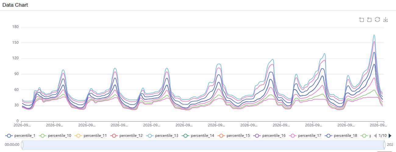
QR AMPS probabilistic forecast showing progressive distribution-cone widening across the 5-day day-ahead forecast horizon
4. Probabilistic Training
The parameters of an AI model are estimated by minimizing a forecasting loss over the training interval. For probabilistic forecasting, however, the training objective differs from that of a conventional point-forecasting model. Rather than estimating only a central value, the training process must learn the conditional behavior of the future value at specified probability levels. Quantile regression provides a practical framework for doing so by directly estimating conditional quantiles of the future value.
4.1 Quantile Loss as the Baseline
The standard starting point for direct quantile forecasting is the asymmetric quantile loss, also known as pinball loss. For quantile level (q), the loss can be expressed as:
Lq(t,h) = q × (Yt+h − Qq(t,h)), if Yt+h ≥ Qq(t,h)
Lq(t,h)= (1 – q) × (Qq(t,h) – Yt+h), if Yt+h < Qq(t,h)
where Yt+his the actual future value and Qq(t,h)is the corresponding quantile forecast.
The asymmetric structure is fundamental to quantile estimation. It causes the training process to penalize errors differently depending on whether the forecast is above or below the eventual observed value. The relative penalty changes with the target quantile (q), allowing the model to learn different quantiles of the conditional forecast distribution.
The pinball loss provides the textbook mathematical baseline for training quantile forecasts and is the starting point for the QR AMPS quantile-forecasting framework.
However, electricity-price forecasting presents additional challenges. Electricity prices can exhibit sharp spikes, heavy-tailed behavior, negative values, regime changes, changing volatility, and highly nonlinear relationships between market, weather, load, generation, congestion, and other explanatory variables. Consequently, applying the standard pinball loss without further adaptation may not provide the required performance across all market conditions. These limitations can be observed empirically when probabilistic forecasting models are applied to actual electricity-price data. In practice, the forecasting implementation must address issues such as:
- Quantile bands can be flat, indicating insufficient differentiation between the estimated quantiles and insufficient learning of the conditional distribution.
- Quantile bands can be too tight, failing to represent sufficient variability in the future price distribution.
- Quantile bands can be symmetrically stacked around P50, failing to capture the asymmetric and transient nature of electricity-price spikes.
- When each quantile is trained independently, lower and higher quantile forecasts can cross, violating the required ordering of the quantiles.
- Built-in probabilistic loss functions can produce substantially different forecast behavior across standard ensemble machine-learning models such as XGBoost, LightGBM, and NGBoost, even when applied to the same forecasting problem.
In light of these issues, QR AI platforms such as QR AMPS and QR ALPS use implementation-specific modifications to the quantile-learning objective and aspects of the training process. These modifications are essential in improving the behavior of probabilistic forecasts, particularly for electricity-price forecasting. The specific modifications are proprietary and are not disclosed in this paper.
4.2 Multi-Quantile Training
QR AI platforms such as QR AMPS and QR ALPS generate multiple quantile forecasts, from 1 to 99, for the same forecast origin t and forecast horizon h. For example, a seven-quantile forecast configuration can be defined as:
𝒬 = {0.05, 0.15, 0.25, 0.50, 0.75, 0.80, 0.95}
The corresponding quantile forecasts are:
𝒬(t,h) = {Q05(t,h), Q15(t,h), Q25(t,h), Q50(t,h), Q75(t,h), Q80(t,h), Q95(t,h) } = {P05, P15, P25, P50, P75, P80, P95}
A general multi-quantile error minimization objective can be represented as:
Ltotal= Σq ∈ 𝒬 wq × Lq(t,h)
where wq represents the relative contribution assigned to quantile q. In the simplest case, the quantiles may receive equal weights. Production implementations can use different weighting schemes depending on the forecasting application and operational requirements.
In standard architectures each quantile forecast corresponds to an individual AI model in terms of both training and execution. In the example above, the seven-quantile configuration therefore involves seven different AI models. The combination of these models must preserve valid quantile ordering and appropriate probabilistic behavior. For example, the seven AI models can be trained and executed as a coordinated model set and, where computational resources permit, in parallel.
Using a 7 or the full 99 quantile models does not necessarily mean that forecast execution takes 99 times longer. With appropriate architecture, the data required by all 99 AI models is loaded once, and the feature engineering is performed once and shared across the AI models, which can then be executed in parallel. The 99 resulting forecasts are written with a single API call to the same data structure. This minimizes redundant data access and API operations and allows computational and data-storage resources to be used efficiently.
4.3 Model Selection
QR AMPS and QR ALPS development continuously evaluate multiple gradient-boosting approaches for probabilistic electricity-price forecasting, including LightGBM, NGBoost, and XGBoost. In empirical testing conducted for price forecasting, these models can produce substantially different quantile price forecasts when using the same features and the same training-data range. The results can further vary across different temporal resolutions, including 5-minute, 15-minute, and hourly price time series.
The precise reasons for these differences have not been established conclusively. Several characteristics of the different boosting frameworks could potentially contribute to the observed differences, including their tree-construction strategies, regularization behavior, histogram-based optimization, treatment of nonlinear feature interactions, and interaction with the quantile-learning objective.
Accordingly, QR AMPS and QR ALPS do not assume that one boosting framework is universally superior for probabilistic forecasting. Model selection is based on empirical performance for the specific forecasting problem, data characteristics, temporal resolution, forecast horizon, quantile levels, and operational requirements. Ultimately, algorithm selection should be based on out-of-sample performance, calibration, robustness, and inference requirements rather than on the algorithm name alone.
5. Probabilistic System Architecture
5.1 Real-Time Probabilistic Forecasting
Real-time probabilistic forecasting introduces engineering challenges in meeting practical user requirements:
- The forecast must be produced while it is still useful to the decision-making process. The model itself is only one part of the latency budget. Data acquisition, feature construction, serialization, database access, quality control, and forecast delivery can materially affect end-to-end execution time.
- High-frequency forecast data must be stored and managed efficiently.
- Multi-quantile forecasts must be displayed at high resolution to allow users to visualize the upper and lower forecast bands.
For example, a 5-min RTD price forecast over a 24-Hour horizon generates 288 forecast points. If we generate 3 quantile forecasts, P05, P50, P95, these amount to 288 x 3 = 864 quantile forecast values executed at each run. To be useful for dispatch decision making, these forecasts have to be reproduced fresh every 5 minutes to adapt to the latest price levels, this means 288 consecutive executions during the 24-hour window, resulting in a total of 248,832 daily quantile forecast points
288 x 864 = 248,832.
Two sets of production level challenges arise that platforms such as QR AMPS and QR ALPS have addressed:
- Forecast generation latency. For an RT 5-minute or 15-minute market, the QR AMPS practical engineering standard is to generate a complete refreshed 24-hour probabilistic forecast within approximately 3 minutes, subject to the market’s actual data and operational constraints. This 3-minute target is an engineering and AI-system architecture requirement, not a mathematical property of probabilistic forecasting. It must be validated under realistic production workloads.
- High-volume probabilistic forecast storage. A probabilistic forecast can generate a large number of output values. In the above example, the 248,832 daily output forecasts are for one RTD node. Typically, a utility may monitor 10 of these, resulting in some 2.5 M forecast points per day. This volume requires an appropriate data architecture for efficient storage, retrieval, indexing, and compression. Production implementations can use techniques such as structured or binary object storage, JSON-based forecast objects where appropriate, hypertable indexing, and different compression or retention strategies for hot and cold forecast data. The specific storage architecture remains proprietary for each platform.
5.2 Designing for Low-Latency Inference
A production grade system such as QR AMPS or QR ALPS should be designed so that the 24-hour forecast horizon is treated as one forecast workload rather than as 288 independent application requests. The objective is to minimize repeated data access, feature computation, model initialization, and database operations across the forecast horizon. Key engineering approaches include:
- Batch model inference where supported. The 288 future forecast intervals can be presented to the AI model as a batch rather than invoking the model separately for each interval. This reduces application-level invocation overhead and allows the underlying inference engine to process multiple forecast intervals efficiently.
- Vectorized feature generation. Features required for the 24-hour forecast should be generated for all forecast intervals as a vectorized operation where possible. This is substantially more efficient than constructing the feature set independently for each of the 288 forecast intervals.
- Caching of inputs that do not change between forecast updates. Many inputs used by the forecasting models do not change during every five-minute refresh. These inputs can be retained in memory or an appropriate intermediate data store and reused rather than repeatedly retrieved or reconstructed.
- Incremental feature updates rather than recomputing the full historical feature set at every update. At each five-minute refresh, only the information that has changed since the previous forecast needs to be updated. Historical observations, derived features, and other state information that remain valid can be retained and reused.
- Efficient model loading and reuse. Model initialization and loading can introduce significant overhead when multiple quantile models are involved. Models should therefore be loaded and retained for reuse where the production architecture permits, rather than repeatedly loading the same model for every forecast interval or every forecast request.
- Compact serialization and database writes. The complete set of quantile forecasts can be serialized as a single forecast object rather than storing every individual forecast value as a separate database record. For example, a BLOB-based storage approach can store the complete set of quantile forecasts as a single JSON object. This can substantially reduce the number of database write operations and associated indexing overhead. The appropriate serialization and storage format depends on the database architecture and downstream query requirements.
- Parallel processing of independent target or model components. Independent quantile models, target variables, nodes, or other computational components can be executed concurrently where sufficient computational resources are available. This is particularly important when multiple quantile models are used for the same forecast horizon.
The practical objective is therefore to reduce the execution time of the entire forecasting data and computational pipeline, not merely to make the machine-learning algorithm itself faster. Data retrieval, feature engineering, model inference, serialization, API operations, and database writes must all be considered when designing the system to meet the approximately 3-minute forecast-refresh requirement.
5.3 Multiple Forecast Band Display
The QR AMPS and QR ALPS user dashboards display realized real-time prices together with probabilistic forecast distributions at the selected forecast resolution. The visualization combines the realized CAISO RTD price with a compact quantile representation that allows users to assess both the central forecast and the uncertainty surrounding it. The quantile visualization uses three selected points from the forecast distribution:
P05 as the low forecast, P50 as the middle or median forecast, and P95 as the high forecast.
The resulting P05–P95 interval is displayed as a vertical blue bar, with P50 representing the median within that interval. The realized CAISO RTD price is overlaid as an orange trace. This allows the user to visually determine whether the realized price falls within the forecast uncertainty range and how it compares with the median forecast.
For example, in the dashboard shown, the forecast was published at 21:51, while the corresponding realized CAISO RTD price was published at 21:53. The realized price falls within the forecast P05–P95 interval, demonstrating that the observed market outcome was contained within the uncertainty range generated by the probabilistic forecast.
This visualization is not intended to show three independent forecasts. Rather, P05, P50, and P95 are quantiles of a single conditional forecast distribution. The P05–P95 range therefore provides a direct visual representation of forecast uncertainty, while P50 provides the central tendency of that distribution.
6. Probabilistic Evaluation
We will discuss three different evaluation concepts quantile loss is not the same thing as calibration or sharpness.
- Quantile loss evaluates the accuracy of quantile forecasts using realized outcomes.
- Calibration evaluates whether the probabilistic statements made by the forecasts correspond to the observed frequencies of those events. For example, a well-calibrated P80 forecast should have the realized future value at or below the P80 forecast approximately 80% of the time over a sufficiently large evaluation sample
- Sharpness describes the concentration of the predictive distribution. A sharper forecast assigns probability to a narrower range of possible outcomes, while maintaining appropriate calibration.
6.1 Calibration
Calibration evaluates whether the stated probability levels correspond to observed frequencies. For example, the P05 and P95 forecasts define a central 90% prediction interval:
I90%(t,h) = [Q0.05(t,h), Q95(t,h)] = [P05, P95]
For each forecast case, the interval is compared with the corresponding realized future value. If the forecast is generated at time ti for horizon hi, the corresponding realized value is Yti+hi.
The empirical coverage of the 90% prediction interval over N forecast cases is:
Coverage90% = (1/N) × NΣi = 1 G(Yti+hi ∈ I90%(ti,hi))
where
- N is the total number of forecast intervals evaluated.
- I90%(ti,hi) is the 90% prediction interval generated for forecast case i.
- Yti+hi is the actual realized future value corresponding to that forecast case.
- G(.) is an indicator function that equals 1 when the realized value falls inside the prediction interval and 0 otherwise.
Example hourly day-ahead forecasts
Suppose a 24-hour DA forecast is generated every day, with 10 quantiles for each hour. For one day, we have 24 forecast intervals, 10 quantile forecasts per interval. Therefore, for coverage evaluation:
N=24
The indicator compares each of those 24 intervals against the actual value that subsequently occurred.
For a 30 day forecast horizon,
N = 30 × 24= 720
A well-calibrated 90% interval should contain the realized observation approximately 90% of the time over a representative evaluation population. Therefore, approximately:
720 × 10% = 72
actual values would be expected to fall outside the 90% prediction interval. More specifically:
- Approximately 36 values (5%) should fall below P05.
- Approximately 36 values (5%) should fall above P95.
- Approximately 648 values (90%) should fall inside the P05–P95 interval.
This is an expected calibration property, not a requirement that exactly 72 observations must fall outside in every 30-day sample. A calibrated model could have, for example, 68 or 77 observations outside the interval due to sampling variation.
Calibration should also be examined by horizon, season, market regime, location, and extreme-event condition. Coverage should not be considered in isolation. Very wide intervals can achieve high coverage while providing limited decision value. Probabilistic quality therefore requires a balance between calibration and sharpness.
In QR AMPS and QR ALPS, quantile forecasting incorporates algorithmic mechanisms for modeling forecast uncertainty across the prediction horizon. These mechanisms allow data scientists to fine-tune the calibration and sharpness of the quantile forecasts discussed in the following sections.
- a) Percentile: one can select the quantile levels: P05, P10, P25, P50, P75, P90, P95. This automatically adjusts the AI engine and the data pipeline.
- b) A dedicated parameter, “Expand forecast uncertainty with horizon,” controls how the width of the probabilistic forecast bands expands as the delivery period moves further into the future.
- c) The “Calibration Points” parameter controls the number of points used in the calibration and probabilistic-learning process. This parameter influences how the quantile forecasts are learned and calibrated across the forecast horizon.
When enabled and appropriately configured for a given time-series type (price, demand, or renewable generation) and resolution (5 to 60 minutes), these parameters control the progressive growth or spread of forecast uncertainty with lead time. This allows the probabilistic forecast to reflect the greater uncertainty generally associated with more distant delivery periods, from a relatively concentrated distribution at shorter horizons to a wider range of plausible future outcomes at longer horizons.
These parameters are configured during the initial model fine-tuning process. Once configured, they are applied to subsequent executions of the probabilistic model.

6.2 Sharpness
Sharpness describes the concentration of the predictive distribution. A sharper forecast assigns probability to a narrower range of possible future values. And this is why a model cannot simply make its P05–P95 interval extremely wide to achieve good coverage: high coverage alone does not mean the probabilistic forecast is informative.
For example, suppose two models both have approximately 90% coverage: Model A has I90%=[90,110], and Model B has I90%=[20,180]. Both could have 90% coverage, but Model A is much sharper because its prediction interval is much narrower.
W90%(h)=Q0.95(h)–Q0.05(h)
Sharpness is fundamentally a property of the predictive distribution itself, not simply a measure of accuracy or narrowness. A narrow predictive distribution is desirable only when it remains appropriately calibrated to the realized outcomes. For electricity-price forecasting, achieving an appropriate level of sharpness may require targeted modifications to the quantile-forecast generation and training process. The objective is not simply to minimize the width of the prediction interval, but to produce a predictive distribution that is both well calibrated and sufficiently sharp for the intended application.
6.3 MAE for the Central Forecast
MAE can be evaluated for the median P50 forecast:
MAE = (1/N) × NΣi = 1 ∣Yi−Q0.50,i∣
6.4 Quantile Loss or Pinball Loss
Quantile Loss or Pinball Loss measures the forecasting error of an individual quantile by comparing the quantile forecast with the corresponding realized value, using the asymmetric penalty appropriate to the specified quantile level, as discussed in 4.1. Let us consider an example:
For a particular forecast case, suppose the model produces
- a P80 forecast:
Q0.80(h)=150
- After the forecast horizon has passed, the actual price is observed:
Yt+h=180
- The standard P80 quantile loss is:
L0.80=0.80 (180-150)=24
Now consider another forecast with the same P80 forecast:
- a P80 forecast:
Q0.80(h)=150
- but the actual price is:
Yt+h=120
- The quantile loss is now:
L0.80 = (1−0.80)(150−120) = 6
The difference between the two penalties is intentional. P80 is a high quantile, so the loss function places a larger penalty on observations occurring above the P80 forecast than on observations occurring below it. The same 30 absolute error produces a loss of 24 when the actual price is above P80, but only 6 when it is below P80. In general we define.
Quantile or Pinball Loss:
Pinball Loss = (1 – q) x | Pq – Yt+h |, if Pq(h) > Yt+h,
Pinball Loss = q x | Pq – Yt+h |, if Pq(h) ≤ Yt+h.
We next review how to evaluate a loss metric for multiple forecast intervals
1. P05 Pinball Loss
| Delivery interval | P05 forecast | Actual price | Loss calculation | P05 loss |
|---|---|---|---|---|
| 10:00–10:15 | $60 | $50 | 0.95 × (60 − 50) | 9.50 |
| 10:15–10:30 | $70 | $90 | 0.05 × (90 − 70) | 1.00 |
| 10:30–10:45 | $55 | $40 | 0.95 × (55 − 40) | 14.25 |
| 10:45–11:00 | $80 | $100 | 0.05 × (100 − 80) | 1.00 |
| Average P05 loss | 6.44 |
2. P50 Pinball Loss
For P50, (q=0.50), so both over forecasting and under forecasting errors receive a weight of 0.50.
| Delivery interval | P50 forecast | Actual price | Loss calculation | P50 loss |
|---|---|---|---|---|
| 10:00–10:15 | $60 | $50 | 0.50 (60-50) | 5.00 |
| 10:15–10:30 | $70 | $90 | 0.50 (90-70) | 10.00 |
| 10:30–10:45 | $55 | $40 | 0.50 (55-40) | 7.50 |
| 10:45–11:00 | $80 | $100 | 0.50 (100-80) | 10.00 |
| Average P50 loss | 8.125 | |||
Average P50 loss = (5+10+7.5+10) / 4 = 8.125
For P95, q = 0.95. Observations above the forecast receive a weight of 0.95, while observations below the forecast receive a weight of 0.05.
| Delivery interval | P95 forecast | Actual price | Loss calculation | P95 loss |
|---|---|---|---|---|
| 10:00–10:15 | $60 | $50 | 0.05 (60-50) | 0.50 |
| 10:15–10:30 | $70 | $90 | 0.95 (90-70) | 19.00 |
| 10:30–10:45 | $55 | $40 | 0.05 (55-40) | 0.75 |
| 10:45–11:00 | $80 | $100 | 0.95 (100-80) | 19.00 |
| Average P95 loss | 9.8125 | |||
Average P95 loss} = (0.50+19+0.75+19) / 4 =9.8125
We can now average the Pinball losses across the 3 quantile forecasts:
| Average P05 loss | Average P50 loss | Average P95 Loss | Overall Mean Quantile Loss |
|---|---|---|---|
| 6.44 | 8.12 | 9.81 | 10.23 |
Mean Quantile Loss = Pinball Loss = (L05 + L50 + L 95) / 3
= ( 6.44 + 8.12 + 10.23 ) / 3 = 8.26
6.5 CRPS
CRPS (Continuous Ranked Probability Score) evaluates the quality of a probabilistic forecast by comparing the entire predictive distribution with the realized future value. Unlike quantile loss, which evaluates one quantile at a time, CRPS assesses the forecast distribution as a whole and therefore provides a single score for each forecast case. Lower CRPS indicates a closer match between the predicted distribution and the realized outcome. CRPS can be useful when comparing different probabilistic forecasting models, although its direct application requires a complete predictive distribution or an appropriate representation of the distribution.
CRPS can also be adapted to a discrete quantile setting such as QR AMPS, where the model produces a finite set of quantile forecasts rather than a continuous predictive distribution. In this case, the predictive distribution can be represented or approximated using the available quantile levels, and the CRPS can be evaluated from the resulting discrete quantile representation. This provides a distribution-level evaluation while remaining consistent with a quantile-based forecasting architecture.
I recommend defining a consistent CRPS approximation for QR AMPS using piecewise-linear interpolation of pinball loss across quantile probabilities, with an explicit rule for the unobserved tails.
This allows you to use different quantile sets for 5-minute forecasts and DAM forecasts while applying the same methodology.
It = N − 1Σi = 1 Lqi,t + Lqi+1,t2 (qi+1 − qi)
To define the treatment of the unobserved tails consistently, use the following convention:
Below the lowest available quantile (q_1),
7. Joint Probability Space
Probabilistic forecasts for electricity prices, ancillary-service prices, and renewable generation are initially generated as individual or marginal predictive distributions. For applications such as co-optimization of trading and bidding, however, the relevant uncertainty is the joint behavior of multiple market variables.
Suppose there are K uncertain forecast variables or market products, such as Energy, RegUp, and Renewable generation. The vector of future outcomes can be represented as:
Yt+h= (Yt+h(1),Yt+h(2),…,Yt+h(K))
where k indexes the forecast variables or products. For example,
Yt+h(Energy),Yt+h(RegUp), Yt+h(RegD)
and additional variables may include other ancillaries, reserves, renewable generation, load, or other quantities relevant to the application.
QR AMPS or QR ALPS produces marginal quantile forecasts for each variable:
Qq(k)(h), or PQ(k)(h), k=1,…,K
Where
- k runs through the number of forecast variables/products forecasts K,
- q runs through potentially different quantile levels selected to predict those products, e.g.,
q∈Q = {0.05, 0.10, 0.25, 0.50, 0.75,0.80, 0.95}.
Recall the marginal quantile forecast is related to the marginal conditional distribution of each variable by:
Pq(k)(h)=Qq(k)(h)=Fk-1(q∣Xt)
where Fk(. ∣Xt)is the marginal conditional distribution of variable k and q runs through the quantile levels. For example,
P50(k)(h)=Q0.5(k)(h)=Fk-1(0.5∣Xt).
Joint Distribution
The future forecast variables can be represented collectively as the vector:
Yt+h= ( Yt+h(1),Yt+h(2),…,Yt+h(K))
The joint conditional distribution of these variables is:
FY(y | Xt ) = P ( Yt+h(1)≤y1 ,…,Yt+h(K)≤yK | Xt)
where y1, …, yK are possible values of the corresponding forecast variables.
The joint CDF can then be evaluated at selected marginal quantile forecasts. For example:
FY(Qq1(1)(h), …, QqK(K)(h) | Xt ) =
P ( Yt+h(1)≤Qq1(1)(h) ,…,Yt+h(K)≤QqK(K)(h) | Xt)
Where
- k runs through the number of forecast variables/products forecasts K,
- q1, …, qK runs through potentially different quantile levels for each product or variables Yt+h. If they all use the same set of quantile levels, we could have:
q∈Q = {0.05, 0.10, 0.25, 0.50, 0.75,0.80, 0.95}.
For an individual product k, the marginal quantile forecast is related to its conditional marginal distribution by:
P ( Yt+h(k)≤Qq(k)(h) | Xt) = q
For example, with two market products:
- k= 2 and market variable Y1= Energy and Y2= RegUp.
- q = quantile level q∈Q = {0.05, 0.50, 0.95}.
By the formula above, the joint distribution function can be evaluated at combinations of marginal quantiles:
P ( YEnergyt+h ≤Qq1Energy(h), YRegUpt+h ≤Qq2RegUp(h) | Xt).
For example, a quantile combination can be q1 = 0.05, and q2 = 0.95:
ω=(Q0.05(Energy)(h),Q0.95(RegUp)(h))
and the corresponding point in the joint probability space is:
P ( Yt+h(Energy) ≤ Q0.05(Energy)(h), Yt+h(RegUp) ≤ Q0.95(RegUp)(h) )
Other combinations are:
ω=(Q0.05(Energy)(h),Q0.05(RegUp)(h))
ω=(Q0.95(Energy)(h),Q0.05(RegUp)(h))
The marginal quantile forecasts describe the uncertainty of each individual variable, while the joint probability distribution additionally describes the dependence between those variables. The important point is that the joint distribution is not generally the product of the two marginal distributions, unless the variables are conditionally independent. For example,
[ P (Yt+h(Energy) ≤ Q0.05(Energy)(h), Yt+h(RegUp) ≤ Q0.95(RegUp)(h) | Xt) ] ≠ 0.05×0.95 = 4.75%.
This distinction is important for applications such as asset optimization, particularly battery bidding and multi-product co-optimization. A battery may simultaneously face uncertainty in Energy prices, ancillary-service prices, and other market variables. The marginal quantile forecasts describe the uncertainty of each variable separately, while the joint probability distribution provides the mathematical framework for representing how those uncertainties occur together.
The joint probabilistic representation therefore provides the foundation for downstream optimization systems such as QR BOSS. The subsequent scenario-generation process can then convert this joint representation into a set of usable future market outcomes for bidding, trading, and co-optimization.
The joint probability representation can be constructed using several statistical and machine-learning approaches. Common approaches include multivariate distribution models, dependence models such as copulas, and scenario-generation or sampling methods. The appropriate method depends on the number of forecast variables, the strength and structure of their dependence, and the required resolution of the resulting probabilistic representation.
8. Applications
8.1 Price Risk
Quantiles provide a compact representation of downside and upside price risk. The same forecast can therefore support bidding, trading, risk analysis, and scenario-based optimization. The P05 and P95 forecasts define a central 90% prediction interval:
I90%(t,h) = [Q0.05(t,h), Q95(t,h)] = [P05, P95]
The lower-tail risk threshold for an energy seller is Q0.05(t,h) = P05 because prices below P05 represent the lower 5% tail of the conditional forecast distribution. Conversely, the upper-tail risk threshold for an energy buyer is Q95(t,h) = P95 because prices above P95 represent the upper 5% tail of the conditional forecast distribution.
These quantiles can therefore be used as inputs to bidding, trading, risk-management, and optimization decisions. The specific interpretation as Value at Risk depends on how the financial loss variable and market position are defined.
8.2 Demand Forecasting Applications
The same probabilistic forecasting framework can be applied to electricity demand, although demand forecasting has different drivers and model behavior from electricity price forecasting. Typical demand-forecasting inputs include temperature, humidity, calendar variables, time of day, historical demand, weather forecasts, renewable generation, distributed energy resources, and system-specific characteristics. The importance of these variables can vary by location, season, customer composition, and operating conditions.
Probabilistic demand forecasts are useful because demand uncertainty changes with operating conditions. Extreme temperatures, unusual load patterns, holidays, renewable variability, and other conditions can result in different levels of forecast uncertainty.
The resulting quantile forecasts can support reserve assessment, dispatch planning, renewable integration, energy procurement, trading, and scenario analysis. They can also support what-if analysis by modifying relevant inputs, such as temperature or renewable generation, and evaluating the resulting changes in the demand forecast.