Single-Family Bottom-Up Demand Type Seasonal Forecasting

Data & Methodology Disclaimer

This case study uses actual, historical, and anonymized energy data for analytical and demonstration purposes. The location, customer segment, dates, and other identifying characteristics have been generalized and are presented as Sample Town.

Although the underlying observations are historical, the analysis applies current AI and machine-learning technology available as of 2026 through QuantRisk’s QR ALPS (AI Load Prediction System). The forecasting workflow uses modern machine-learning libraries and techniques for feature engineering, model configuration, optimization, training, and forecast evaluation.

The historical dataset provides a consistent real-world environment for examining electricity-demand behavior, including seasonal effects, weather sensitivity, time-of-day patterns, and differences between consumer segments. The purpose is not to represent current market conditions, but to demonstrate how modern AI methods can learn from and forecast established energy-consumption patterns.

Quantitative results are reported only where supported by the underlying analysis.

1. The Case

Accurate electricity demand forecasting is essential for energy companies, utilities, aggregators, and other organizations that need to anticipate consumption, optimize operations, manage supply and demand, and reduce forecasting risk.

For this case study, the objective was to develop an AI-powered load forecasting solution for Sample Town, focusing on electricity consumption across Single Family Residences customers. The forecasting task was designed to predict the final week of each season, using the historical hourly demand and relevant external variables available before the forecast period.

Rather than relying on a single deterministic forecast, the solution was designed around an AI-driven forecasting workflow capable of learning recurring consumption patterns, incorporating weather and calendar effects, and producing forecasts that can be extended to probabilistic predictions and uncertainty intervals.

The solution was implemented using QR ALPS, covering the forecasting workflow from data preparation and exploratory analysis through feature engineering, model configuration, training, validation, forecasting, and monitoring.

The case demonstrates how an end-to-end AI forecasting platform can transform historical energy data into actionable forecasts for operational and planning decisions.

2. The Data

The forecasting solution uses a proprietary historical dataset containing anonymized hourly electricity consumption data for Sample Town.

The dataset was intentionally frozen for this case study so that the forecasting problem could be evaluated under controlled historical conditions. The final week of each season was treated as the forecast horizon, while the preceding historical observations were used for model development, experimentation, and validation.

2.1 Input Data

The forecasting workflow integrates several categories of data:

• Historical electricity consumption: Hourly Single Family Residences load/demand observations for Sample Town.
• Weather data: Hourly regional weather observations, with particular emphasis on variables such as temperature and humidity.
• Calendar information: Holidays and other calendar characteristics relevant to Single Family Residences consumption.
• Time-based information: Hour of day, day of week, weekday/weekend classification, and seasonal characteristics.

2.2 Forecast Output

The primary output of the AI forecasting system is the forecast values for the target period.

The combination of demand history, weather, calendar information, and temporal features allows the AI models to distinguish between recurring consumption patterns and external factors that influence electricity demand.

For example, the system can identify differences between:

• Weekdays and weekends
• Working days and holidays
• Morning and evening demand peaks
• Seasonal consumption patterns
• Weather-driven changes in electricity usage

This provides a stronger foundation for forecasting than relying solely on historical load values.

3. Data Exploration and Pattern Discovery

Before configuring the forecasting models, the data science team conducted an extensive exploratory analysis to understand the underlying behavior of electricity consumption.

This step is critical in energy forecasting because demand is rarely random. It typically contains multiple interacting patterns, including daily, weekly, seasonal, calendar, and weather-driven effects.

Using data analysis and visualization capabilities within the forecasting workflow, the team examined the historical hourly consumption data and identified recurring behavioral patterns across the four seasons.

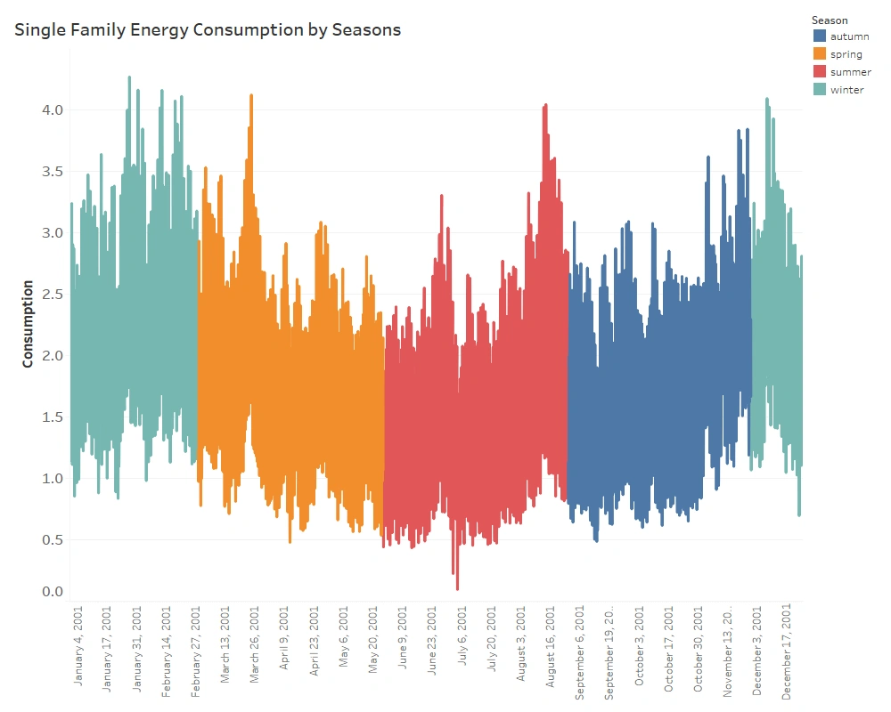
For the purposes of this case study, the year was divided into:

• Spring: March 1 – May 31
• Summer: June 1 – August 31
• Autumn: September 1 – November 30
• Winter: December 1 – February 28

The final week of each season was reserved as the forecasting target.

Importantly, the forecasting workflow did not simply train a model and immediately produce the final forecasts. Historical periods corresponding to previous seasonal forecast horizons were used for model experimentation, validation, and error analysis.

This allowed the team to compare alternative model configurations and identify the feature and model settings that were most appropriate for the forecasting problem before applying the finalized configuration to the target periods.

3.1 Seasonal Behavior — Spring

The first stage of analysis focused on identifying the consumption characteristics of the Spring period.

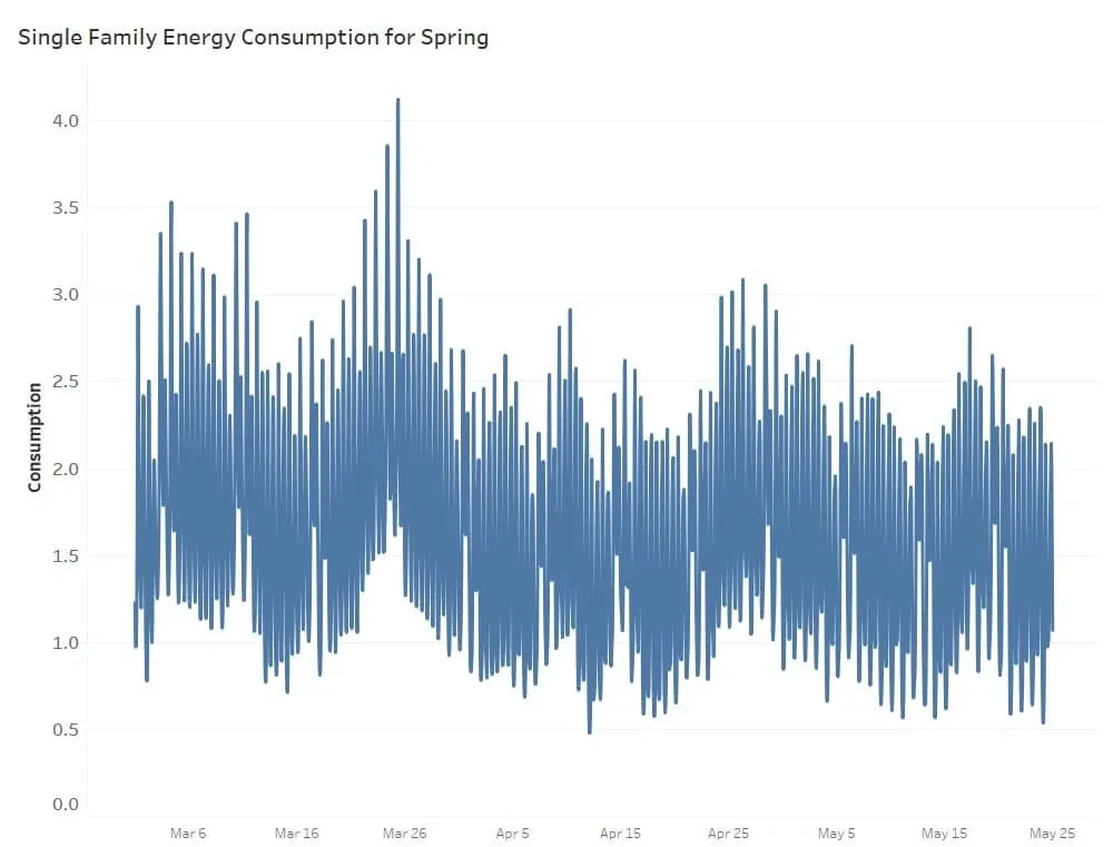
Analysis of the hourly Single Family Residences electricity data revealed clear intraday patterns, including recurring morning and evening demand peaks.

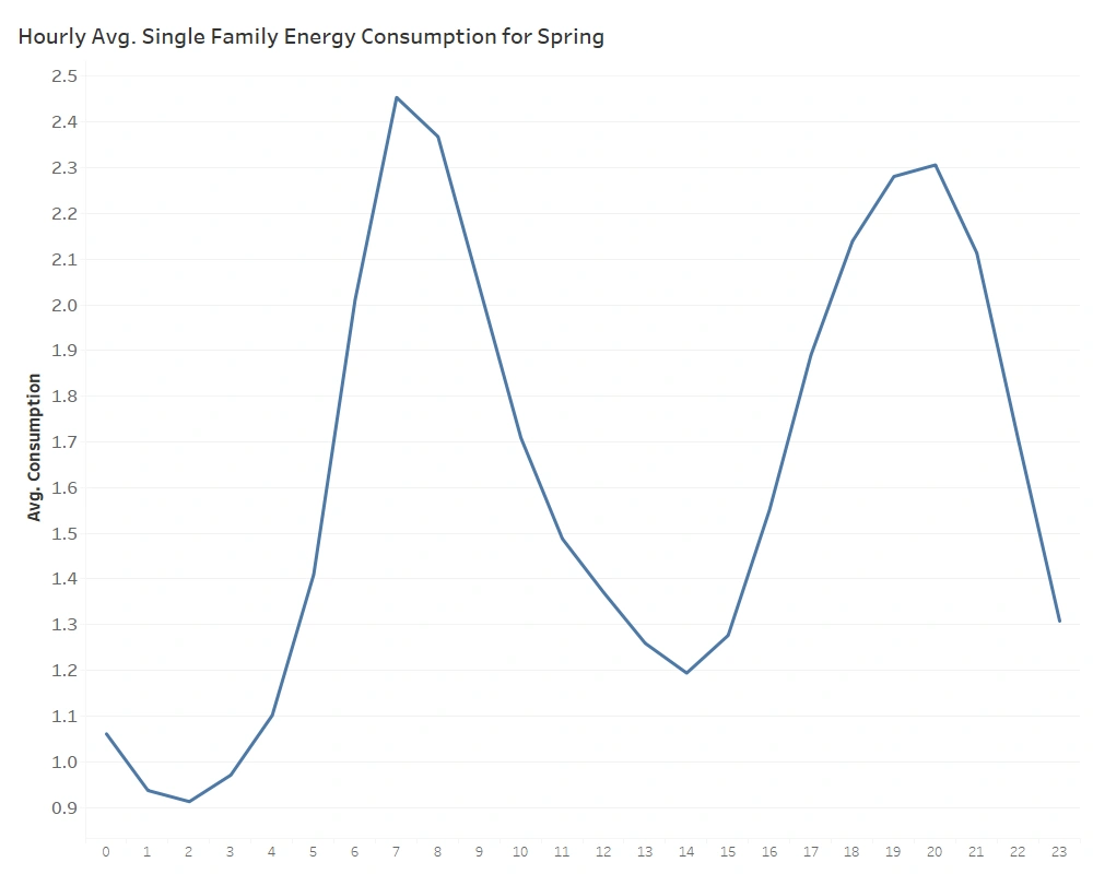
The data showed two major consumption periods during a typical day:

• A morning demand increase, beginning in the early morning and continuing through the morning peak.
• An evening demand increase, beginning in the late afternoon and continuing into the evening.

The analysis indicated that consumption was strongly dependent on the hour of the day, making time-of-day information an important predictor for the AI models.

Key Observations

The Spring analysis identified several important patterns:

• Two recurring daily demand peaks were visible in Single Family Residences electricity consumption.
• Morning demand began increasing during the early morning hours and reached a peak during the morning period.
• A second increase occurred during the late afternoon and evening.
• Demand behavior varied significantly throughout the day.
• The consumption profile therefore could not be adequately represented without capturing hourly temporal behavior.

These observations directly informed the feature-engineering strategy discussed hereunder.

3.1.1 Weekday vs. Weekend Behavior

The analysis was further refined by examining hourly consumption separately across the days of the week.

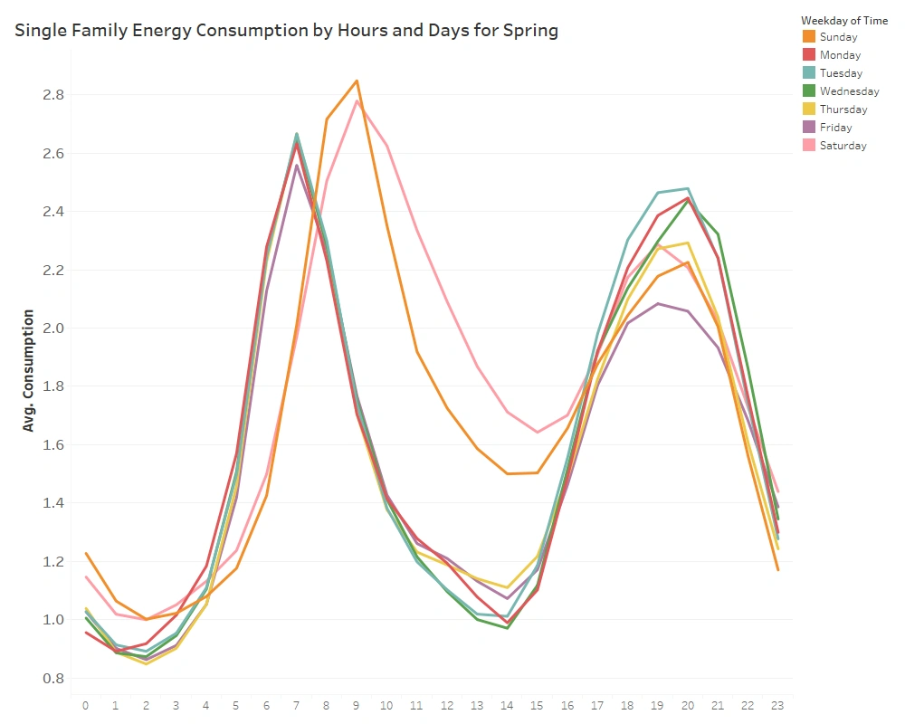
This analysis demonstrated that Single Family Residences demand patterns were not identical throughout the week.

Weekday Behavior

• During weekdays, the data showed relatively consistent daily patterns, including recognizable morning and evening peaks.
• The middle of the day generally exhibited lower Single Family Residences consumption, consistent with changes in household occupancy and daily routines.

Weekend Behavior

Weekend consumption followed a different profile.

The demand pattern showed:

• Different timing of peak consumption
• Higher consumption during certain daytime periods
• Different morning and evening demand characteristics
• Less pronounced midday reduction compared with typical weekdays

These differences are particularly important for machine-learning-based forecasting because a model that treats every day as statistically identical may fail to capture systematic behavioral changes.

3.1.2. Feature Engineering Implications

The weekday/weekend analysis reinforced the importance of including:

• Day-of-week features
• Weekend indicators
• Calendar variables
• Hour-of-day features

within the forecasting model.

These variables allow the AI system to learn that, for example, an 8:00 AM observation on a Saturday may have a fundamentally different expected demand profile from an 8:00 AM observation on a Tuesday.

3.2. Seasonal Behavior of Data — Summer

The next stage of the analysis focused on the Summer consumption profile in Sample Town.

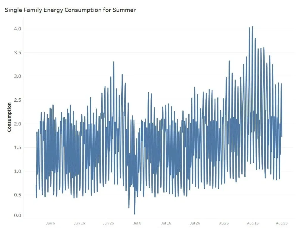
The hourly consumption data was analyzed to identify recurring daily patterns, peak and off-peak periods, and differences between weekday and weekend behavior. This analysis helped determine which temporal features should be incorporated into the AI forecasting models.

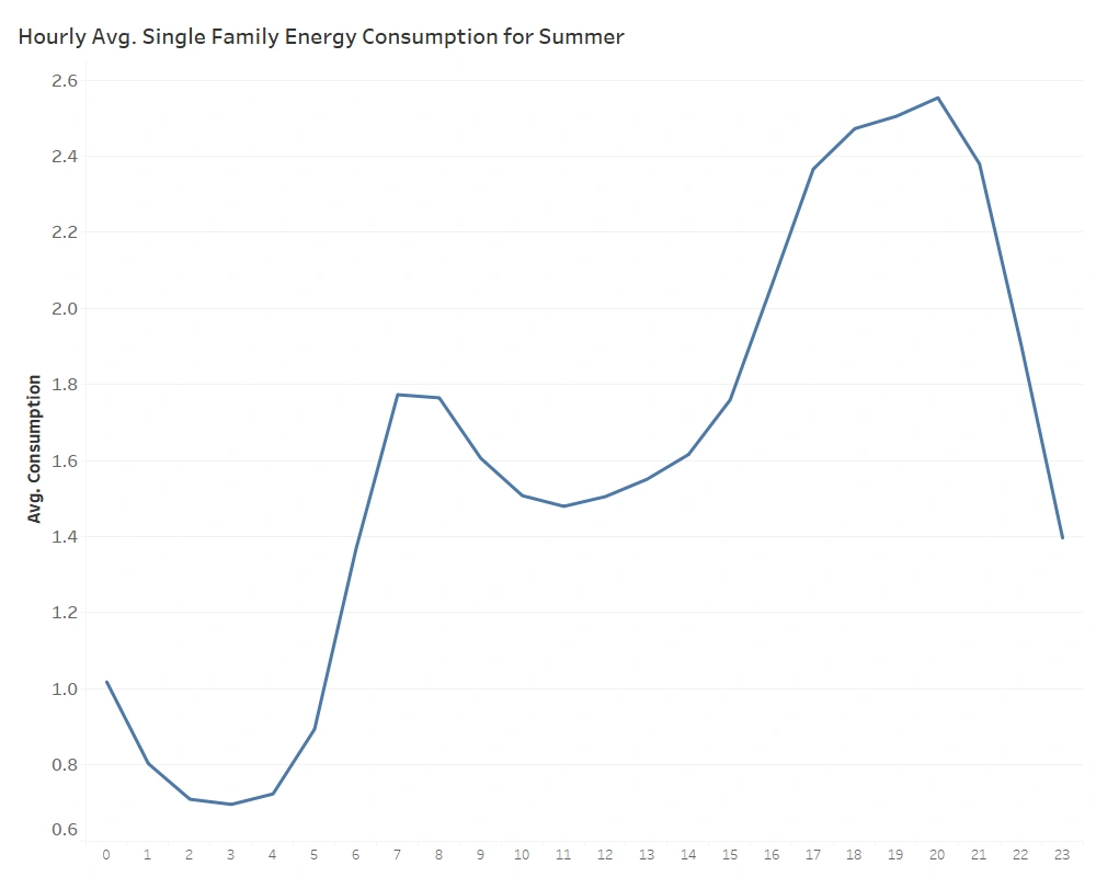
The hourly averages across the Summer training period revealed a recurring two-peak daily profile.

Key Observations

The analysis identified several consistent characteristics:

• Two primary demand peaks occur during a typical day.
• Consumption begins increasing during the early morning hours and continues toward the morning peak.
• A second increase begins during the late afternoon and continues into the evening.
• Peak periods generally occur during the morning and evening.
• Electricity consumption is strongly dependent on the hour of the day.

These observations confirmed that time-of-day information should be explicitly represented within the forecasting model.

3.2.1. Weekday vs. Weekend Behavior

The analysis was further refined by examining the average hourly profile for each day of the week.

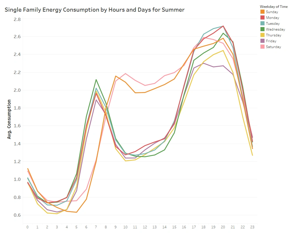
The results indicated that:

• Weekdays follow a relatively consistent pattern with recognizable peak and off-peak periods.
• Morning and evening peaks are more clearly defined during working days.
• Weekend consumption follows a different behavioral profile, with changes in both consumption levels and peak timing.
• Weekend demand tends to remain higher during certain daytime periods than during typical working days.
• The midday reduction in demand observed during weekdays is less pronounced on weekends.

These differences demonstrate why a forecasting model should distinguish between working days, weekends, and holidays, rather than treating every day as equivalent.

3.2.2. Feature Engineering Implications

The Summer analysis reinforced the following feature configuration:

• Hour of day to capture intraday consumption patterns.
• Day of week / weekday to represent weekly behavioral cycles.
• Weekend and calendar indicators to capture systematic changes in Single Family Residences consumption.
• Model Splitter where appropriate, allowing QR ALPS to create and train separate models for different portions of the daily demand profile.

The objective of this configuration is to allow each model to specialize in a particular consumption regime rather than forcing a single model to represent substantially different patterns throughout the day.

3.3. Seasonal Behavior of Data — Autumn

The same analytical process was applied to the Autumn period.

The objective was to determine whether the behavioral patterns identified in other seasons remained stable or whether seasonal changes required adjustments to the forecasting configuration.

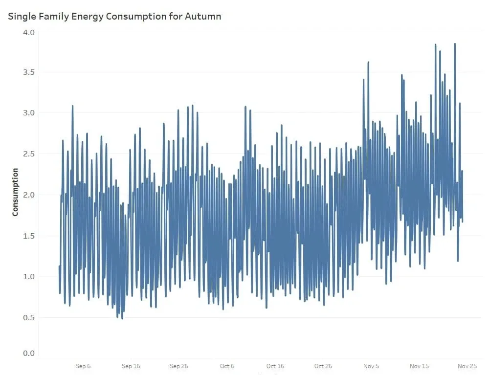
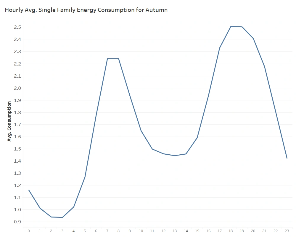
Analysis of the hourly consumption averages showed that the overall Single Family Residences demand profile continued to exhibit recurring morning and evening peaks.

Key Observations

The Autumn data indicated:

• Two primary daily demand peaks.
• A morning increase in consumption beginning during the early hours.
• A second increase beginning during the late afternoon.
• Recurring morning and evening peak periods.
• Strong dependence on the hour of the day.

Although the general daily structure remained recognizable, seasonal conditions and external variables could influence the level and shape of the demand profile.

This reinforced the need for the forecasting system to combine historical consumption patterns with external predictors rather than relying solely on time-based features.

3.3.1. Weekday vs. Weekend Analysis

The day-of-week analysis again revealed meaningful differences between working days and weekends.

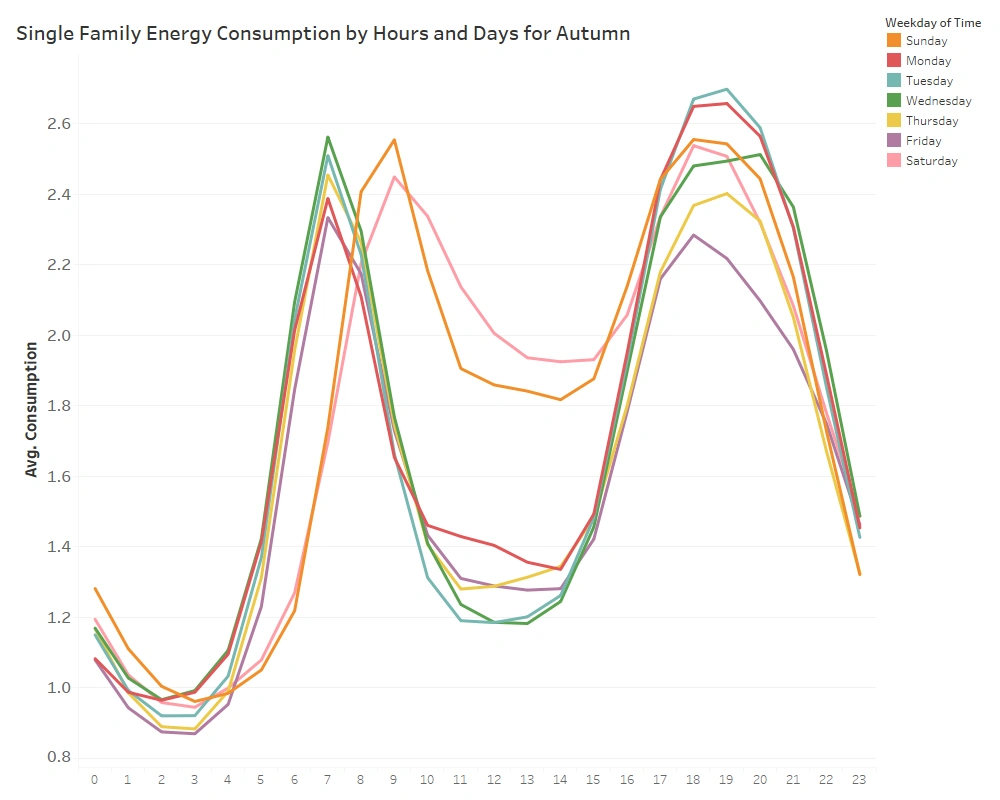
The observed patterns included:

• Weekdays showed relatively consistent demand behavior.
• Morning and evening peaks were more structured during working days.
• Weekend consumption followed a different daily profile.
• Weekend peak periods occurred at different times compared with weekdays.
• Midday consumption was generally lower on working days than during weekends.
• The difference between weekday and weekend profiles remained an important source of predictive information.

3.3.2. Feature Engineering Implications

The Autumn analysis therefore supported the continued use of:

• Hour-of-day features
• Weekday/day-of-week features
• Weekend indicators
• Calendar and holiday features
• Historical load information
• Weather-related external predictors

The Model Splitter configuration could again be used to separate different intraday demand regimes and allow multiple specialized models to be trained within the overall forecasting workflow.

3.4. Seasonal Behavior of Data — Winter

Winter presented another opportunity to examine whether the established demand patterns remained consistent under different seasonal conditions.

The Winter analysis covered the available historical observations from the beginning and end portions of the seasonal period, with the final forecast horizon reserved for evaluation.

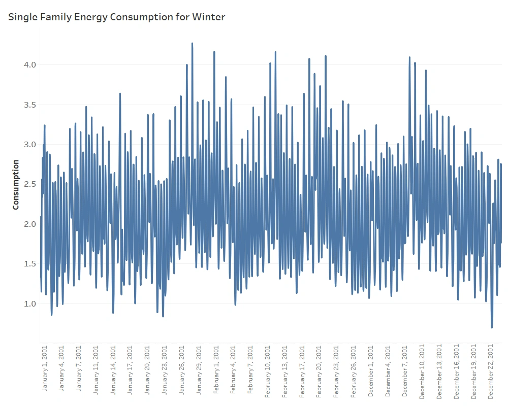
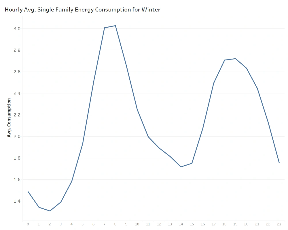
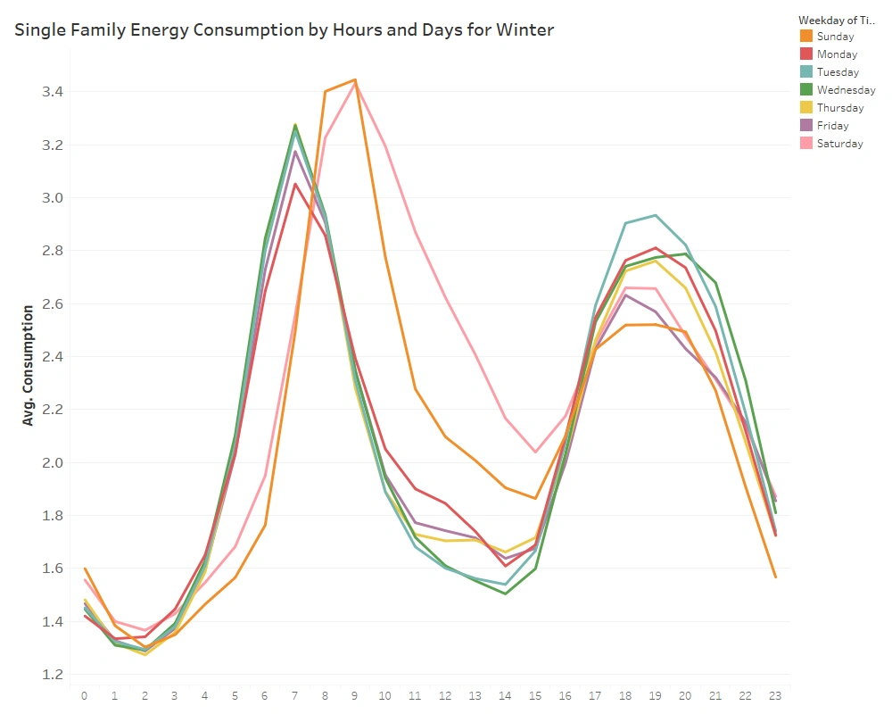
The hourly consumption profile continued to demonstrate clear intraday structure.

Key Observations

The analysis identified:

• Two recurring daily demand peaks.
• A morning increase in Single Family Residences electricity consumption.
• An afternoon and evening increase.
• Distinct peak and off-peak periods.
• Strong dependence on the hour of the day.

The persistence of these patterns across seasons demonstrated the importance of temporal features in the AI forecasting configuration.

At the same time, the overall consumption level and response to external conditions can vary by season. This is why the model architecture combines temporal patterns with external variables such as weather and calendar information.

3.4.1. Weekday vs. Weekend Analysis

The Winter day-of-week analysis showed similar behavioral differences:

• Working days displayed relatively consistent consumption profiles.
• Morning and evening peaks were more structured on weekdays.
• Weekend consumption followed a different pattern.
• Weekend peak timing differed from typical working days.
• Midday demand was generally lower on weekdays.
• Weekend demand remained comparatively higher during portions of the daytime period.

3.4.2. Feature Engineering Implications

The Winter analysis confirmed the continued relevance of:

• Hour of day
• Day of week
• Weekend indicators
• Calendar and holiday information
• Historical demand patterns
• Weather variables

The Model Splitter capability could again be configured to allow specialized models to learn different portions of the daily demand curve.

4. Feature and Correlation Analysis

After identifying the primary temporal patterns, the next step was to determine which external variables could provide additional predictive information.

In energy forecasting, historical demand alone may not fully explain changes in consumption. Weather, solar conditions, calendar effects, and other external variables can influence both the level and shape of electricity demand.

The data science team therefore performed correlation and behavioral analysis between the historical Sample Town electricity consumption series and available external time series.

The purpose was not simply to select variables with a high statistical correlation, but to identify external predictors that could provide meaningful information about seasonality, intraday behavior, and changes in demand levels.

The analysis highlighted several potentially valuable external predictors.

4.1. Factoring in Temperature

Temperature is an important variable in electricity demand forecasting because changes in ambient conditions can influence household electricity usage.

The analysis compared electricity consumption patterns with available temperature observations across different periods and seasons.

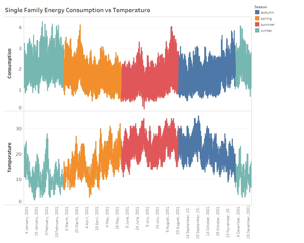
The results indicated that temperature provided information about changes in the consumption profile and could therefore help the forecasting model distinguish between otherwise similar time periods.

Conclusion

• Temperature should be considered as an external feature/predictor in the AI forecasting model.
• Including temperature enables the model to use observed or forecast weather conditions when estimating future demand, helping it adapt the expected consumption level to changing environmental conditions.
• Where sufficient data is available, additional weather-derived variables such as apparent temperature or cooling/heating indicators can also be evaluated during model optimization.

4.2. Factoring in Solar Radiation

Solar radiation data was also analyzed as a potential external predictor.

Variables such as:

• DHI — Diffuse Horizontal Irradiance
• DNI — Direct Normal Irradiance
• GHI — Global Horizontal Irradiance

provide information about solar conditions throughout the day.

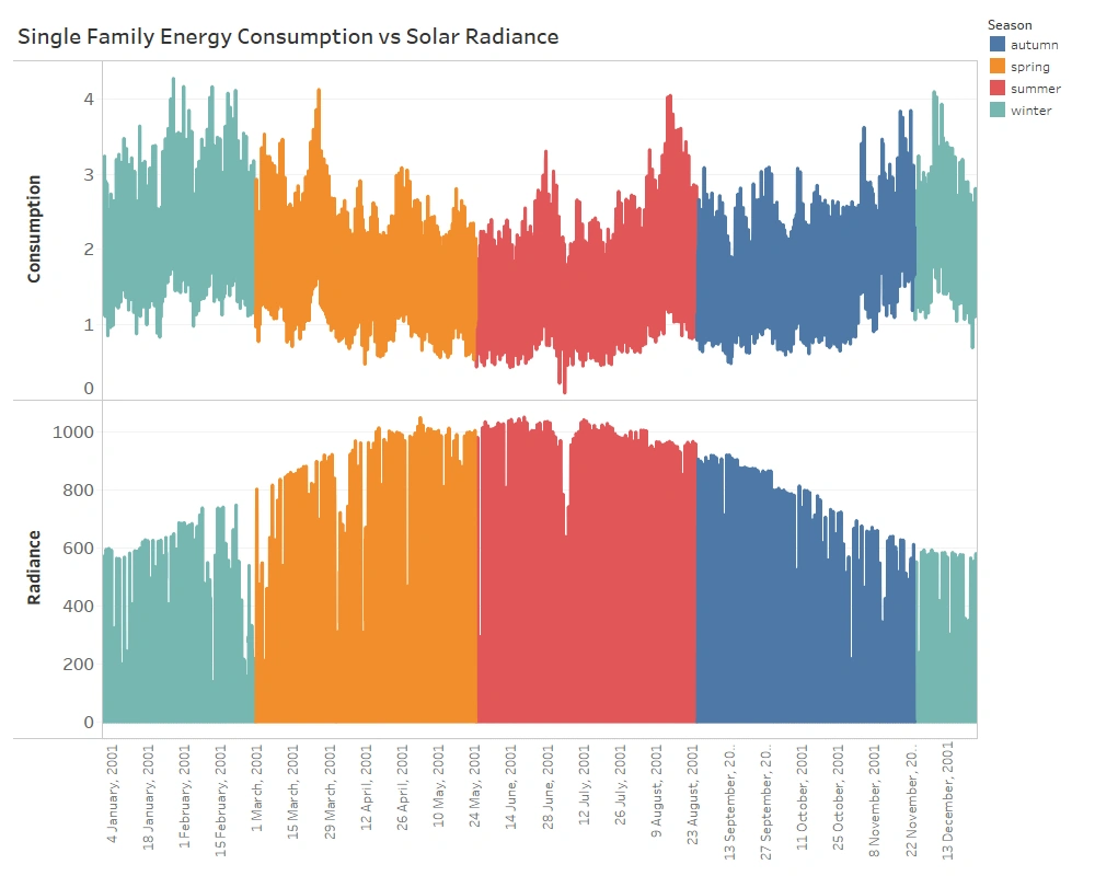
The intraday behavior of these variables can help identify changes associated with daylight and seasonal conditions.

Conclusion

Solar radiation variables can be included as external predictors where the underlying data demonstrates useful predictive relationships with demand.

These features can help the AI model capture:

• Intraday changes
• Daylight-related patterns
• Seasonal changes
• Variations in environmental conditions

Their final inclusion should be determined through model validation and feature-importance analysis rather than correlation alone.

4.3. Factoring in Humidity

Relative humidity was also investigated as a potential predictor of electricity demand.

The analysis indicated that humidity exhibited relationships with changes in the observed consumption profile during different periods.

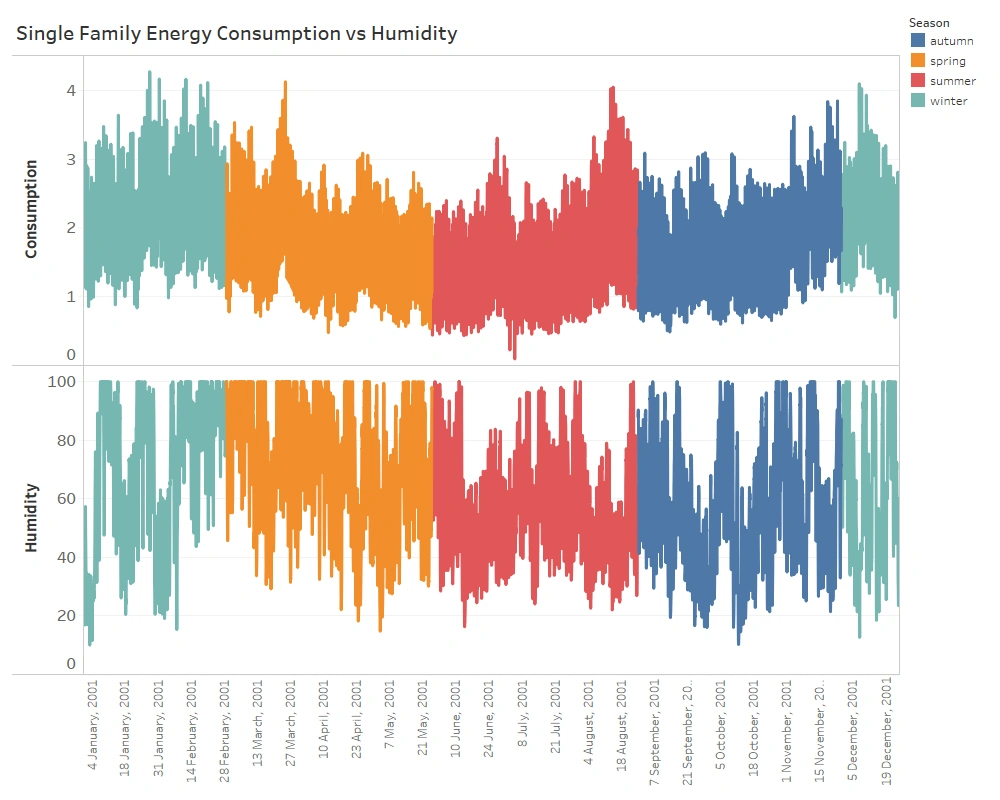
Because humidity can interact with temperature and perceived environmental conditions, it may provide additional information that is not fully represented by temperature alone.

Conclusion

Relative humidity should be evaluated as an external feature/predictor in the AI forecasting model.

Its contribution can then be assessed through model optimization and validation to determine whether it improves out-of-sample forecasting performance.

5. The AI Forecasting Model

Following the data exploration, seasonal analysis, and feature investigation, the next stage was to configure and train the AI forecasting models for Sample Town.

The solution was implemented using QR ALPS, an automated, no-code AI forecasting platform that enables data scientists and energy professionals to configure forecasting workflows through an interactive modeling environment.

The platform brings together data preparation, feature engineering, model configuration, optimization, forecasting, and visualization within a single workflow.

Although the forecasting configuration differed between seasons where necessary, the overall architecture remained consistent.

The forecasting workflow included:

Historical Data → Data Preparation → Feature Engineering → Model Configuration → Automated Optimization → Training → Forecast → Accuracy Analysis

5.1. Data Preprocessing

The first stage of model configuration involved preparing the historical time series for machine-learning-based forecasting.

Gap Filling

Energy time series can occasionally contain missing observations caused by data collection or transmission issues.

QR ALPS provides several gap-filling approaches, including methods based on:

• Linear interpolation
• Daily patterns
• Weekly patterns
• Other time-series characteristics

The historical dataset used in this case contained no significant missing-data problem. Nevertheless, gap-filling capabilities were configured as part of the broader forecasting workflow to make the model more robust to potential data-quality issues.

Calendar Processing

Calendar information was incorporated into the forecasting pipeline to distinguish between:

• Working days
• Weekends
• Holidays
• Other calendar-related demand patterns

This is particularly important for Single Family Residences load forecasting because electricity consumption can change substantially on holidays and non-working days.

The calendar processor allows the model to treat these days differently during training and forecasting rather than assuming that every calendar day follows the same behavioral pattern.

5.2. Feature Engineering

The feature-engineering configuration was derived from the exploratory analysis and correlation studies described above.

Depending on the seasonal forecasting model, the configuration included combinations of:

• Previous-day demand patterns
• Previous-week demand patterns
• Hour-of-day information
• Day-of-week information
• Calendar and holiday indicators
• Temperature
• Humidity
• Solar radiation variables
• Moving-average features

Different lag configurations were evaluated for the individual seasonal models.

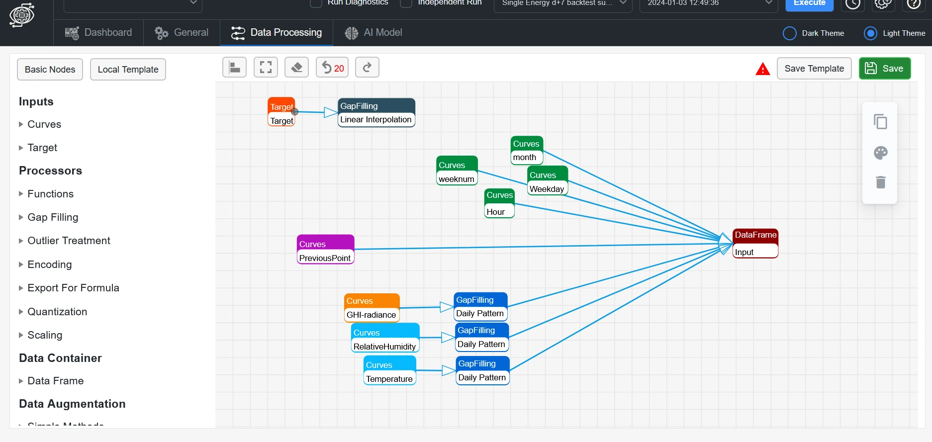
This allowed the forecasting workflow to determine which historical observations contained the most useful information for predicting the target period.

The objective was not to maximize the number of predictors, but to identify a feature set that provided useful predictive information while maintaining robust out-of-sample performance.

5.3. AI Model Configuration

Model Splitter

The Model Splitter capability allows the forecasting workflow to divide the data into different behavioral segments and train separate models for those segments.

For this case, the daily demand profile was divided into three broad periods:

• Midnight to 5:00 AM
• 5:00 AM to 2:00 PM
• 2:00 PM through the remainder of the day

The rationale was based on the exploratory analysis, which showed that different portions of the day exhibited different demand characteristics.

Rather than requiring a single model to learn the entire daily profile, the Model Splitter allows each model to specialize in its corresponding consumption regime.

This approach is particularly useful when a time series contains distinct behavioral patterns across different hours of the day.

5.4. Automated Model Optimization

Multiple machine-learning approaches were evaluated as part of the model-development process.

The forecasting workflow included models such as:

• NGBoost
• LightGBM
• XGBoost

These models can be configured with different hyperparameters and feature combinations to optimize forecasting performance.

For example, an XGBoost configuration can involve parameters such as:

• Booster
• Number of estimators
• Maximum depth
• Minimum child weight
• Gamma
• Maximum delta step
• Subsample
• L1 regularization
• L2 regularization
• Base score
• Evaluation metric
• Objective function

Manually testing every possible combination quickly becomes impractical.

For example, evaluating five candidate values across 12 independent hyperparameters would result in a very large search space.

QR ALPS‘s automated optimization capabilities are designed to address this problem by systematically evaluating model configurations and identifying promising combinations without requiring manual testing of every parameter combination.

This automated process helps reduce the risk of:

• Underfitting, where the model fails to capture important demand patterns.
• Overfitting, where the model performs well on historical training data but poorly on unseen periods.

The exact optimization strategy and computational requirements depend on the model, dataset, search space, and configuration.

5.5. Model Training and Execution

Once the model configuration was finalized, the selected machine-learning models were trained using the historical hourly electricity consumption data for each seasonal forecasting period.

The original case study reported that training and forecast execution for a seasonal dataset of approximately three months of hourly observations took around one minute under the tested configuration and environment.

This execution time is specific to the historical case-study setup and should not be interpreted as a guaranteed runtime for other datasets or production environments.

For production deployments, execution time will depend on factors such as:

• Dataset size
• Number of features
• Number of models
• Optimization configuration
• Forecast horizon
• Hardware and cloud environment

6. Forecasting and Accuracy Analysis

Once the AI models were trained, the resulting forecasts were evaluated through the forecasting and visualization dashboards.

The objective was to assess how effectively the models reproduced historical demand behavior and to generate the final forecasts for the reserved seasonal forecast horizons.

6.1. Forecast Visualization Dashboard

QR ALPS provides interactive visualization capabilities that bring together forecast results and model-performance information.

The analysis included:

• Actual demand
• Forecast demand
• Forecast errors
• MAE – Mean Absolute Error
• MAPE – Mean Absolute Percentage Error

These metrics provide complementary views of forecasting performance.

MAE measures the average absolute difference between actual and forecast values, while MAPE expresses the average absolute error relative to the actual value.

The dashboards allow users to move beyond a single summary metric and inspect forecast behavior at individual timestamps.

This is important in energy forecasting because an acceptable average error can still conceal significant errors during specific peak-demand periods.

6.2. Reported Forecast Accuracy

For the historical Sample Town case, the reported error are displayed below:

Spring

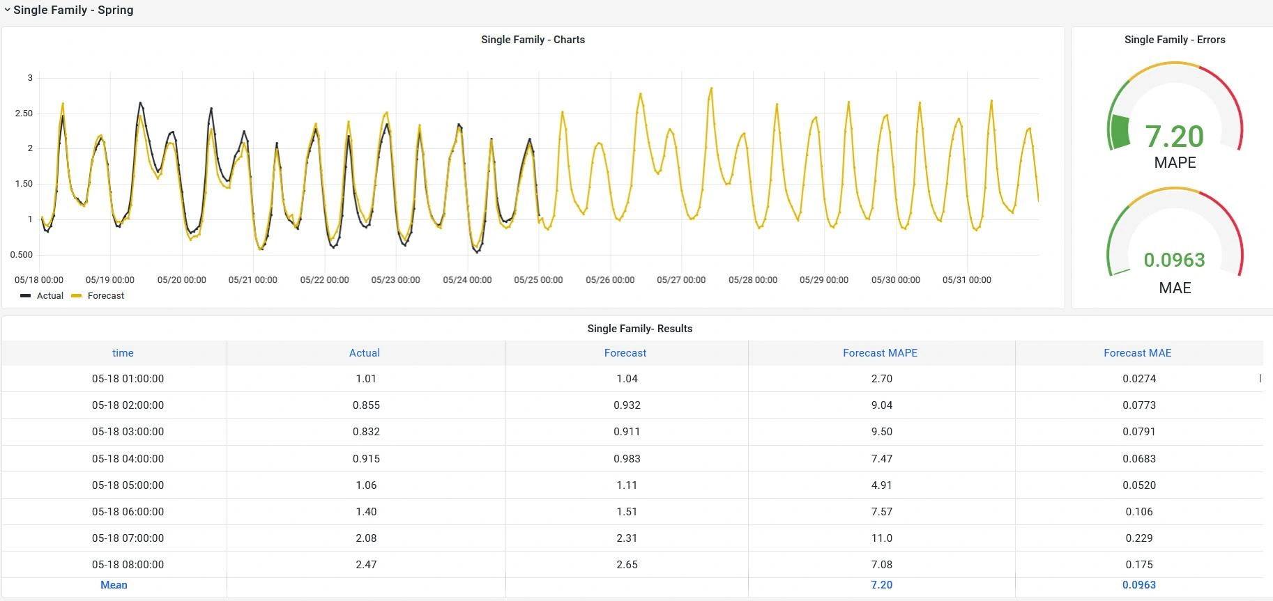
[QR ALPS Data Visualization Dashboard, Actual, Forecast and Accuracy Hourly Data. May 18th – May 31st.]

Summer

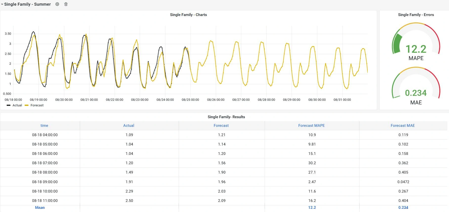
[QR ALPS Data Visualization Dashboard, Actual, Forecast and Accuracy Hourly Data. Aug 18th – Aug 31st.]

Autumn

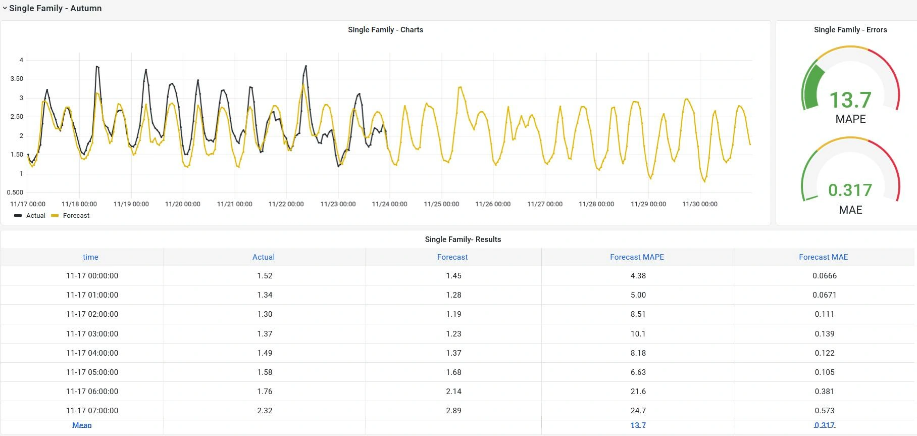
[QR ALPS Data Visualization Dashboard, Actual, Forecast and Accuracy Hourly Data. Nov. 17th – Nov. 30th.]

Winter

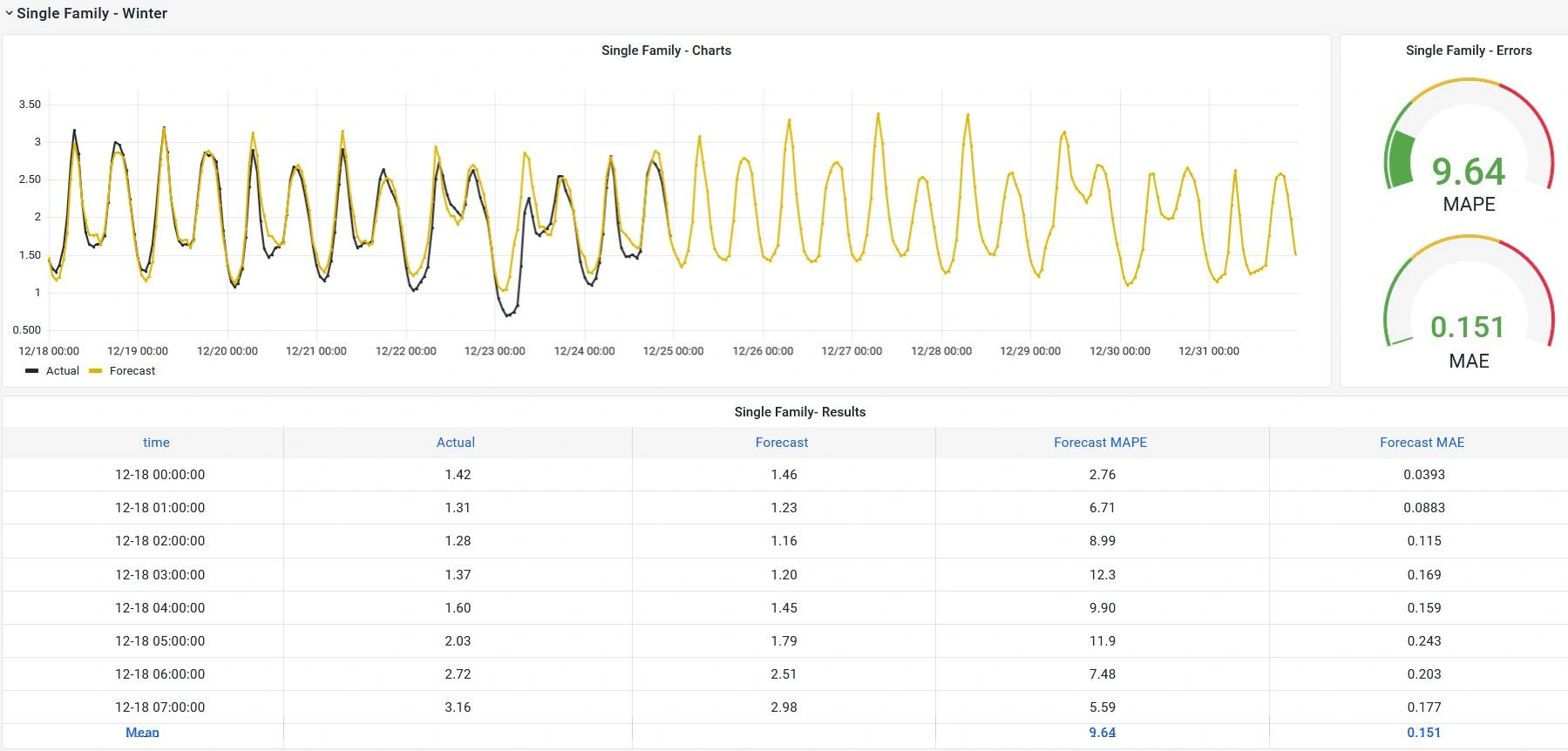
[QR ALPS Data Visualization Dashboard, Actual, Forecast and Accuracy Hourly Data. Dec.18th – Dec 31st.]

These figures represent the results reported for this particular historical dataset, model configuration, forecast horizon, and evaluation methodology.

They should therefore be interpreted as case-specific results rather than guaranteed performance benchmarks for other customers, geographies, datasets, or forecasting horizons.

The variation between seasons also illustrates an important characteristic of energy forecasting: forecasting difficulty can change depending on the stability and predictability of the underlying consumption profile.

7. Scenario Simulation and Future Planning

Once a forecasting model has been established, the same framework can be extended beyond a single baseline forecast.

Scenario simulation can be used to investigate questions such as:

• What happens if temperature increases significantly?
• How could different weather conditions affect demand?
• What would demand look like under alternative calendar assumptions?
• How sensitive is expected consumption to changes in external variables?
• What range of demand should operational teams prepare for?

This transforms the forecasting system from a tool that simply predicts “what is likely to happen” into a decision-support capability that can help organizations explore “what could happen.”

For energy companies, utilities, aggregators, and other market participants, this distinction is important because operational decisions are often made under uncertainty rather than around a single expected value.

8. End-to-End AI Forecasting Capability

The Sample Town case illustrates an end-to-end forecasting workflow rather than an isolated machine-learning model.

The complete process can be summarized as:

1.  Data Integration
   Connect historical load, weather, calendar, and other relevant data sources.
2.  Data Quality
   Identify gaps, anomalies, inconsistencies, and other data-quality issues.
3.  Data Exploration
   Analyze daily, weekly, seasonal, and external-variable relationships.
4.  Feature Engineering
   Create temporal, lagged, calendar, weather, and other predictive features.
5.  AI Model Selection
   Evaluate appropriate machine-learning algorithms for the forecasting problem.
6.  Automated Optimization
   Tune model parameters and configurations using historical validation.
7.  Forecast Generation
   Produce hourly demand forecasts for the target horizon.
8.  Probabilistic Forecasting
   Where configured, quantify forecast uncertainty through prediction intervals and distributions.
9.  Monitoring
   Continuously compare forecasts with actual outcomes and track model performance.
10.  Interactive Visualization
    Provide operational users with dashboards for forecasts, actuals, errors, and trends.
11.  Scenario Simulation
    Evaluate alternative future conditions and their potential impact on demand.

This end-to-end approach provides a foundation for moving from a one-time forecasting study toward a scalable, continuously monitored AI forecasting operation.