1. Introduction
1.1 Context & Purpose
Electricity and gas demand forecasting becomes materially more difficult when the objective extends beyond predicting raw hourly MW values to explaining the structural composition of load and isolating its weather sensitivity.
This decomposition is particularly critical across large, geographically diverse footprints characterized by distinct climatic conditions, customer mixes, and load profiles. The Midcontinent Independent System Operator (MISO) footprint, spanning ten Local Resource Zones (LRZs) from the Canadian border down to the Gulf Coast, provides an ideal test case. MISO’s own planning and operational frameworks recognize the necessity of evaluating LRZs independently because regional demand drivers vary significantly across the footprint.
Isolating weather-driven load components within observable net-load data is essential for Load Serving Entities (LSEs), utilities, distribution system operators (DSOs), and retail energy providers (REPs). Clear structural visibility directly informs power sourcing, day-ahead and real-time scheduling, imbalance management, and peak load contribution (PLC) planning. Key operational questions include:
- Scenario Analysis: How does predicted load shift under relative temperature variations (e.g., +2°F or -5°F against baseline forecasts)?
- Base Load Baseline: What portion of the forecasted demand is purely temperature-independent (baseload)?
- Cooling vs. Heating Sensitivity: What proportion of the load is driven by cooling demand versus heating demand?
- Regional Heterogeneity: How do weather-sensitive load components differ across distinct LRZs?
- Aggregation Mechanics: How does weather-sensitivity behavior change when aggregating from an individual LRZ up to the system-wide MISO footprint?
- Path Dependency: How do short-term shifts in temperature trajectories impact peak load timing and magnitude?
- Uncertainty Quantification: How does weather uncertainty propagate into final load forecast variance?
1.2 The Structural Shift in MISO
These questions are increasingly vital as the MISO grid evolves. MISO’s long-term resource planning highlights geographically differentiated load growth driven by data center development, industrial expansion, electric vehicle (EV) adoption, distributed energy resources (DERs), and space heating electrification (such as heat pumps). A robust decomposition framework separates weather-driven volatility from fundamental base-load trends without assuming all load changes are weather-induced.
This case study uses public demand data from MISO to add precision in the model. However, the methodology and processes apply directly to any load serving entity or grid and distribution system operating in similar climates.
1.3 The Technical Modeling Challenge
The primary modeling challenge arises because a single, static temperature variable fails to capture actual load behavior:
- Non-Linearity: A 10°F temperature shift produces radically different MW impacts depending on the season, time of day, and geographic zone.
- Thermal Asymmetry: The load response to cooling demand (Cooling Degree Hours / CDH) differs fundamentally in shape and scale from heating demand (Heating Degree Hours / HDH).
- Thermal Inertia & Path Dependency: Weather effects are cumulative. Several consecutive hours of extreme heat or cold alter building thermal dynamics differently than an isolated, short-duration temperature spike.
To address these challenges, an effective load model must isolate weather-sensitive demand as explicit, interpretable components within the net-load signal, rather than treating weather as a black-box feature. The model must accurately calibrate parameters against historical interval data and enable deterministic and probabilistic scenario forecasting across arbitrary weather paths. The QR AI Load Prediction System (QR ALPS) was designed to solve this structural decomposition challenge. The platform is used as the analytic driver of this case study
2. Mathematical Load Model and Methodology
2.1 Weather Transformations: Degree-Hour Mechanics
A foundational principle in advanced load modeling is that raw ambient temperature readings cannot be directly ingested into a linear model without losing structural fidelity. The temperature Td.t on a day d, at hour t must first be transformed into directional, non-linear variables Heating Degree Hours (HDH) and Cooling Degree Hours (CDH) that directly map to building thermodynamics and human comfort responses:
- HDHd,t : Heating Degree Hour representing the heating-sensitive component
HDHd.t = max (0, HTbase – Td.t )
with HTbase,t (Heating Base Temperature): The thermal turning point below which space heating systems activate (typically near 68°F).
- CDHd,t : Cooling Degree Hour representing the cooling-sensitive component;
CDHd.t = max (0, Td.t – CTbase )
with CTbase,t (Cooling Base Temperature): The thermal turning point above which air conditioning systems activate (typically near 72°F).
Key Modeling Insights:
- Asymmetric Deadband: For context, MISO’s published market analysis uses a 65°F base temperature for its HDD/CDD calculations. This may be fine for reporting style analysis. However, from an actual model implementation perspective, QR ALPS states that it is critical to maintain HTbase and CTbase as separate, independent parameters, driven by actual local temperature and demand data, rather than forcing a single, unified reference temperature. The gap between HTbase and CTbase represents a thermodynamic “deadband” where neither heating nor cooling is required. This separation opens the way to an algorithmic mechanism to enforce dynamic seasonal and operational separation within the model parameters. The net result is that the one HDH and CDH estimation algorithm can dynamically adapt itself to different locations, seasons and demand behavior.
- Parameter Invariance: While HTbase and CTbase do not vary by hour or day type, as they define physical equipment activation thresholds, their exact values vary substantially across the ten MISO Local Resource Zones (LRZs) due to temperature effects, regional building codes, insulation standards, and heating fuel mix (gas vs. electric heat pumps).
- Automated Calibration: Platforms like QR ALPS dynamically estimate optimal HTbase and CTbase parameters for each LRZ and sub-zone during automated model calibration against historical interval data.
2.2 The Mathematical Demand Model
Observable meter demand is inherently a net-load signal, representing gross consumer demand offset by Behind-the-Meter Photovoltaic (BTM PV) generation. The structural linear model for net load at day d and hour t is expressed as:
Ld,t = ad,t + bd,t CDHd,t+ cd,t HDHd,t − BTM PVd,t
where
- d is the day and t the hour.
- Ld,t : observed net load (in MW).
- ad,t : Base load representing the temperature-independent demand component, driven by consumer schedules, diurnal human activity, day-of-week patterns, and baseline economic activity.
- Td.t : the temperature on day d, at hour t.
- CDHd,t : Cooling Degree Hour representing the cooling-sensitive component;
CDHd.t = max (0, Td.t – CTbase )
CTbase,t is the cooling base temperature turning point where cooling begins
- bd,t : Cooling sensitivity coefficient (MW/CDH)
- HDHd,t : Heating Degree Hour representing the heating-sensitive component
HDHd.t = max (0, HTbase – Td.t )
HTbase,t is the heating base-temperature turning point where heating begins
- cd,t : Heating sensitivity coefficient (MW/HDH).
- BTM PVd,t represents behind-the-meter photovoltaic generation that reduces observed net load. Typically, BTM PVt = dt GHIt where GHI stands for Global Horizontal Irradiance.
Note: While BTM PV is an essential component of observed net load, its specialized modeling mechanics are covered in a dedicated companion study. This paper focuses strictly on the structural decomposition of weather-sensitive components HDH and CDH.
Transitioning from Daily Parameters to Diurnal Profiles
In a practical production environment, estimating a unique parameter set for every individual day d is mathematically ill-conditioned and leads to severe over-fitting. To make the model operationally viable for forward-looking forecasting, the explicit daily index d is suppressed, yielding a diurnal (hourly) profile model:
Lt = at + bt CDHt + ct HDHt − dt GHIt
Here, parameters at, bt , ct, vary by hour of the day t and seasonal/day-type state.
Standard estimation approaches (such as Ordinary Least Squares or simple multi-linear regression) frequently fail when fitting this model across multi-regional footprints. Naive regressions introduce severe numerical instabilities, such as producing non-zero heating coefficients (bt > 0) during mid-summer peak hours or non-zero cooling coefficients (ct > 0) during freezing winter periods. QR ALPS overcomes this via constrained optimization algorithms and structural regularization, enforcing physical plausibility across all hours.
2.3 Demand Model Parameters and Sensitivity
Let us consider again the net load model
Lt = at + bt CDHt + ct HDHt − dt GHIt
Taking the partial derivatives of the net-load model yields the marginal physical sensitivities of demand with respect to weather and solar inputs:
- Marginal Cooling Sensitivity Coefficient (MW per unit degree of cooling)
bt = ∂Lt / ∂CDHt
- Marginal Heating Sensitivity Coefficient (MW per unit degree of heating)
ct = ∂Lt / ∂HDHt
- Marginal Solar Sensitivity Coefficient (MW per unit irradiance)
dt = ∂Lt / ∂GHIt
Resolving Estimation Instabilities
When calibrating these parameters on historical interval load and weather data, standard statistical methods suffer from collinearity, seasonal transition noise, and data sparsity at temperature extremes. This manifests as:
- Spurious Sensitivities: Detecting unphysical cooling sensitivities in deep winter or heating sensitivities during summer heatwaves.
- Diurnal Discontinuities: Erratic hour-to-hour jumps in bt or ct that violate the physical thermal inertia of building stock.
QR ALPS resolves these issues by applying multi-stage, domain-aware analytical and machine learning frameworks. By coupling algorithmically enforced parameter constraints with seasonal regime-switching rules, QR ALPS ensures that estimated sensitivity coefficients remain smooth, physically realistic, and robust across any MISO LRZ.
2.4 What-If Temperature Scenario Analysis
First the parameters at, bt , ct, dt of the net load model are estimated on recent historic data
Lt = at + bt CDHt + ct HDHt − dt GHIt.
The structural model serves as an engine for temperature scenario analysis, both on historic and forward forecast load.
A baseline historic or forecast load Lt is observed or generated under a primary temperature, risk managers must quantify how demand shifts under severe cold snaps or unexpected heatwaves. For example, if the temperature gets colder by 10 degrees, how much would the demand forecast change?
Recall
bt = ∂Lt / ∂CDHt —> ΔL = bt * ΔCDHt. (2.a)
ct = ∂Lt / ∂HDHt —> ΔL = ct * ΔHDHt. (2.b)
The incremental demand change under the temperature scenarios:
Δ L scenario+10,t = bt * ΔCDH scenario+10,t(2.c)
Δ L scenario-10,t = ct * ΔHDH scenario-10,t(2.d)
Where the
ΔCDH scenario+10,t = (CDHscenario+10,t – CDHBaseline,t ) (2.e)
ΔHDH scenario-10,t = (HDHscenario-10,t – HDHBaseline,t ) (2.f)
The MW impact of the load L under the weather scenarios at time t :
Lscenario+10,t = LBaseline,t + Δ L scenario+10,t (2.g)
Lscenario-10,t = LBaseline,t + Δ L scenario-10,t (2.h)
Worked Operational Example
- Target Interval: Day-Ahead, Hour Ending 19:00 (7:00 PM).
- Baseline AI Load Forecast FLt: 450 MW.
- Baseline Vendor Temperature Forecast: 45°F.
- Calibrated Model Parameters: CTbase = 71°F, HTbase = 65°F, c19 = 12 MW/HDH.
Scenario Query: How does the load forecast change if the ambient temperature drops by 10°F, from 45° to 35°F?
- Baseline HDH (45°F) = max( 0, 65 – 45 ) = 20 HDH
- Scenario HDH (35°F) = max( 0, 65 – 35 ) = 30 HDH
- ΔHDH change of temperature -10 degree = Scenario HDH – Baseline HDH = 30 – 20= 10 HDH.
Equation (2.d) determines the impact of the temperature drop on the demand
Δ L change of temperature -10 degree = 12 * 10 MW = 120 MW.
Equation (2.e) is used as follows:
Scenario Load Forecast (35F) = Base Load Forecast (45F) + ct ΔHDH
= 450 MW + 12 * 10 MW = 570 MW.
The 120 MW shift represents a 26.7% demand increase driven strictly by space heating activation. By explicitly isolating the c19 (12 MW/HDH) rate of change of demand per unit HDH, QR ALPS enables energy traders, LSE risk managers, and grid operators to instantaneously re-run load profiles under arbitrary weather paths without requiring full end-to-end model re-training.
3. MISO LRZ 2-7 Market Case Study
3.1 MISO LRZ 2-7
MISO is divided into 10 Local Resource Zones, which sit within the broader MISO market footprint. MISO defines LRZ boundaries using factors including Local Balancing Authority boundaries, state boundaries, transmission interconnections, resource adequacy studies, relative zone size, and market-seam considerations.
This segmentation matters for load forecasting because weather exposure and demand structure are not spatially uniform. The same weather can affect multiple LRZs while producing different demand responses. Conversely, two LRZs can experience different temperature regimes during the same operating day.
As mentioned before it is valuable that the demand forecasting platform used for analysis be similar to QR ALPS, capable to model all LRZs without having to access and modify the model parameters
- This study focuses on LRZ 2-7, covering a large population footprint of 14.5 million covering Michigan and Wisconsin. This zone is a very good candidate for winter versus summer demand case study, capturing the lake-effect climate extremes of two heavily populated Great Lakes states.
- For temperature data it is preferable to combine DTW (Detroit Metropolitan Airport) and MKE (Milwaukee Mitchell International Airport) temperature as a population weighted average. QR ALPS allows to make a temperature index such as
LRZ 2-7 Temperature = 0.65 * Temperature DWT + 0.35 * Temperature MKE
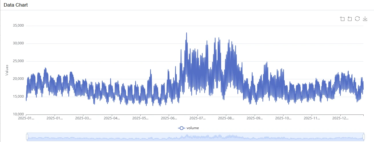
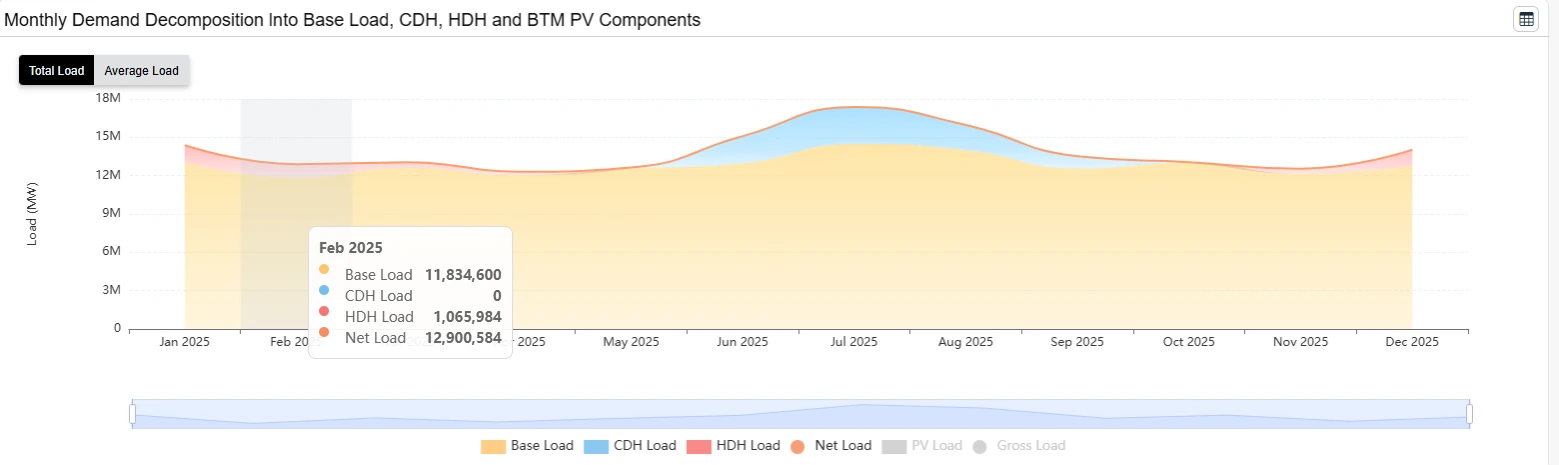
As seen in the plot below, the peak load period of the year 2025 is in summer, July and August.
3.2 LRZ2-7 Base Heating and Cooling Degrees
This case study uses MISO LRZ2-7 load and corresponding temperature composite index data for 2025. The qualitative nature of the findings remain true for other years and zones. The analysis covers the periods:
- HDH analysis, sensitivity rate and MW in January 2025
- CDH analysis, sensitivity rate and MW in August 2025
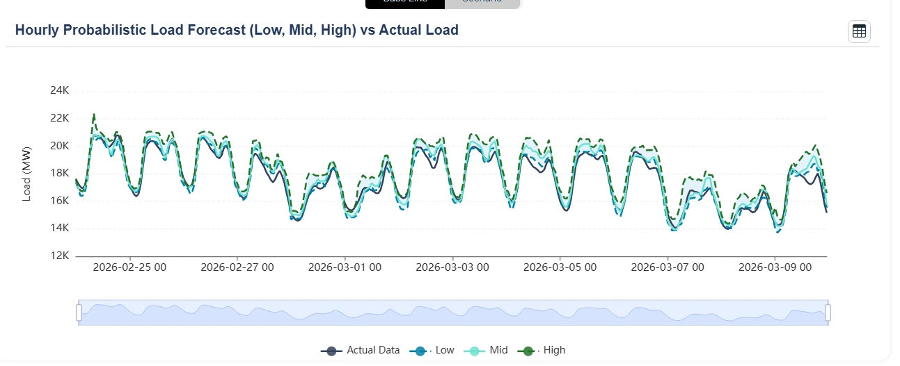
- A 14-DA AI demand forecast from February 24, 2026 to March 9, 2026
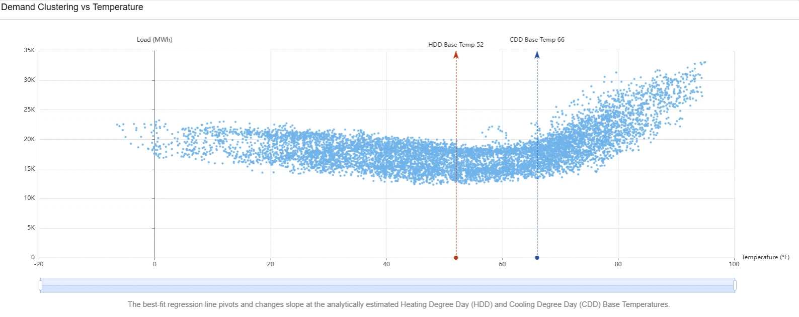
The estimation of the model parameters by QR ALPS yields the MISO LRZ2-7 Base Temperatures:
- HTbase : Heating Base Temperature, the thermal turning point below which space
heating systems activate, 52 F.
- CTbase : Heating Base Temperature, the thermal turning point below which space
heating systems activate. 66 F.
The estimated base temperatures clearly illustrate the turning point where heating and cooling begin. These are perfectly represented in the scatter plot below illustrating the clustering and nonlinear response of LRZ2-7 demand across the temperature range in 2025.
The stacked chart below shows the monthly total decomposition of LRZ2-7 net-demand, as estimated by QR APLS load model, into the weather-insensitive Baseload (in orange color), the heating-sensitive components HDH (in peach) in the two extremes, January to April, and October to December, and the more pronounced cooling-sensitive components CDH (in blue) from June to September. The following two sections examine the heating and cooling sensitivity effects in greater detail, including their relationship with degree-hour conditions and their corresponding MW contribution to net load. QR ALPS runs the same model and analysis live for other LRZ zones. Contact QuatRisk for access to the web portal.
4. MISO LRZ2-7 Winter Demand & HDH Analysis
4.1 Data Analysis
To isolate space heating sensitivity during winter months, QR ALPS, as discussed in Section 2.2 of the Methodology, evaluates the heating-sensitive component of net load:
- at : Base Load representing the temperature-independent demand component, driven by consumer schedules, diurnal human activity, day-of-week patterns, and baseline economic activity.
- HDHt : Heating Degree Hour representing the heating-sensitive component
HDHt = max (0, HTbase – Tt )
where Tt is the temperature at the hour t.
- HTbase : Heating Base Temperature, the thermal turning point below which space
heating systems activate, 52F.
- ct : Heating sensitivity coefficient of the (MW/HDH). The partial derivative of net load per HDH, that is the MW change in net load per 1 unit of HDH. During winter peak days, the diurnal response coefficient ct varies by hour. Night and midnight (hours ending to 20:00 – 04:00) exhibit significantly higher MW sensitivity per degree drop than day periods, reflecting residential heating schedules and commercial building warm-up cycles.
As mentioned in Section 3.1, QR ALPS is used to estimate the parameters of the load model using LRZ2-7 demand data and population weighted temperature index DTW (Detroit Metropolitan Airport) and MKE (Milwaukee Mitchell International Airport).
QR ALPS provides detailed demand decomposition analysis, separating net load into its structural base-load component and weather-sensitive heating and cooling components. The table below presents the demand decomposition at the peak-load hour of selected winter months, including the calculated Heating Degree Hours (HDH) and the resulting heating-sensitive load component.
| Date (Winter Months) | Net Load Peak Hour | Base Load at | Heating Sensitivity Coefficient ct | HDHt oF | HDH (MW) | Net Load (MW) |
|---|---|---|---|---|---|---|
| 2025-01-21 | 18:00 | 19,411.54 | 74.50 | 51.23 | 3,816.65 | 23,228.19 |
| 2025-02-18 | 19:00 | 19,126.16 | 69.48 | 42 | 2,918.1 | 22,044.26 |
| 2025-12-15 | 18:00 | 19,535.18 | 90.81 | 30.35 | 2,756.12 | 22,291.3 |
QR ALPS plots the net load and its decomposition into structural and weather-sensitive components at hourly granularity throughout the month. The MW quantities shown in the table are extracted directly from the corresponding hourly decomposition chart. The chart can be zoomed to examine any individual interval.
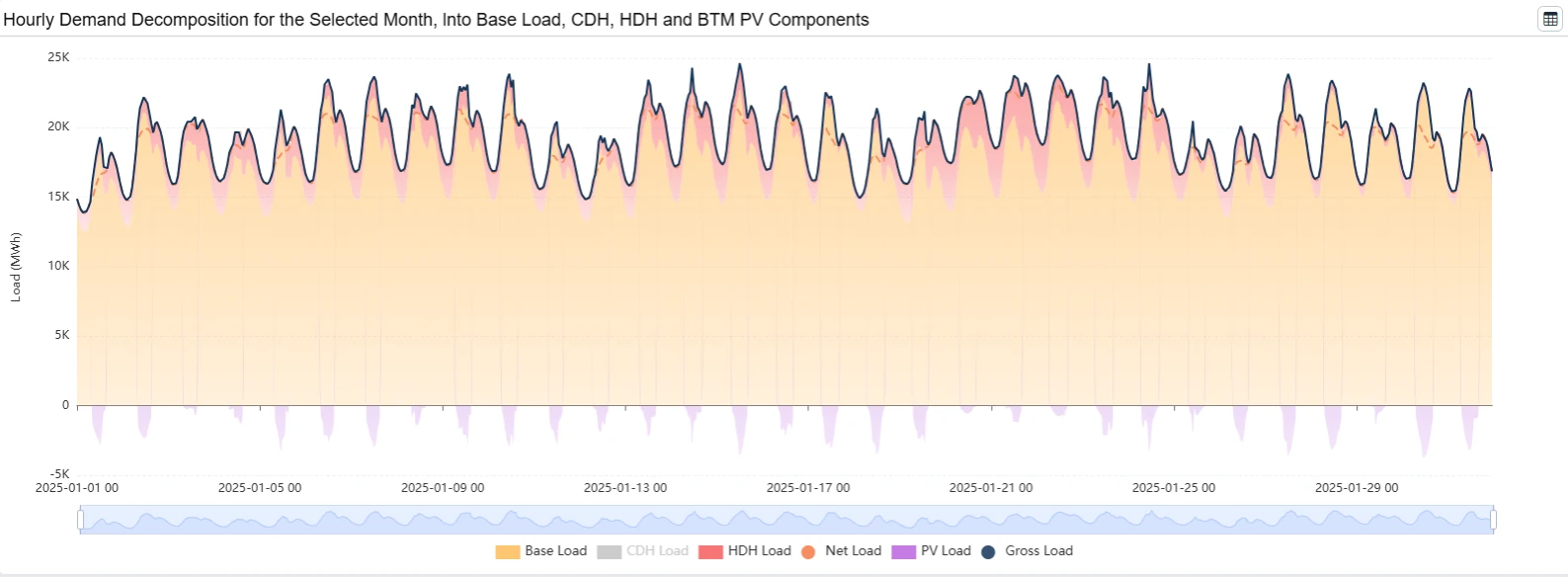
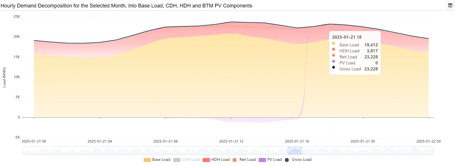
The chart tooltip displays the individual demand components and their contribution to total net load. For the 18:00 interval on January 21, the decomposition is:
| Base Load at | HDH (MW) | Net-Load (MW) |
|---|---|---|
| 19,411.54 | 3,816.65 | 23,228.19 |
Note that the Net-Load is the sum of the Base Load and HDH components. We next discuss these values.
4.2 QR ALPS Heating Decomposition Methodology
4.2.1 Heating Sensitivity Coefficient
As discussed in Section 2, the QR ALPS load model estimates and displays the parameters and quantities used in the load decomposition through multiple reports. This provides full visibility into how the heating-sensitive component is derived.
The heating sensitivity coefficient, ct, is estimated from the historical 2025 load-temperature data. It represents the estimated marginal change in load, in MW, associated with one additional Heating Degree Hour (HDH) at a given interval.
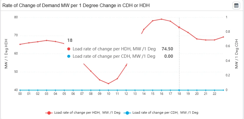
To stabilize the estimation, QR ALPS scales, filters, and aggregates the estimated coefficients to derive a calibrated monthly diurnal heating-sensitivity profile, which is presented in the corresponding report. This calibrated monthly diurnal profile serves as the lookup table used to convert HDH into the heating-sensitive MW component of demand.
For the 18:00 interval in January, the calibrated coefficient is:
c18 = 74.50.
4.2.2 Calculation of HDH
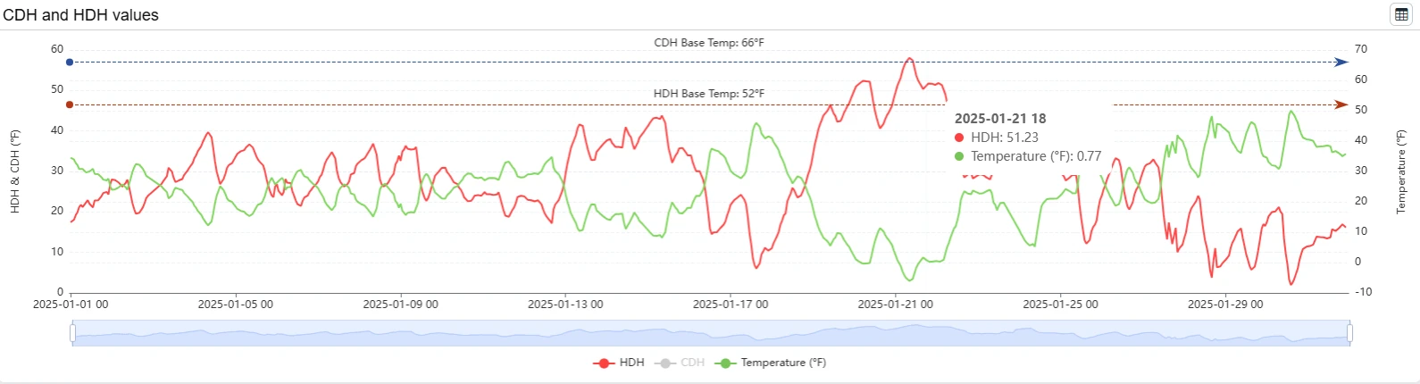
The next step is to calculate the Heating Degree Hours for the specific interval 18:00 on January 21,
- The calibrated heating base temperature is: HTbase = 52 F.
- The temperature is: Tt = 0.77 F.
- Applying the HDH transformation, the Heating Degree Hour for this interval are:
HDHt = max (0, HTbase – Tt ) = max (0, 52 – 0.77) = 51.23
4.2.3 Calculation of the Heating-Sensitive MW Component
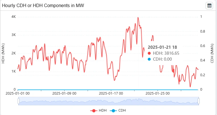
The heating-sensitive component of net load, L(HDH,t), is then calculated using the calibrated heating sensitivity coefficient. This is accomplished by the load model formula discussed in section 2.2:
L(HDH,t) = ct * HDHt = 51.23 * 74.50 = 3,816.65 MW
The resulting 3,816.65 MW is the model-driven heating-sensitive component of the net load at 18:00 on January 21.
4.2.4 Application to Forecasting
The above calculation illustrates how QR ALPS performs hourly demand decomposition. The key model parameter is the calibrated monthly diurnal heating-sensitivity coefficient, which captures how load responds to heating conditions at each hour of the day.
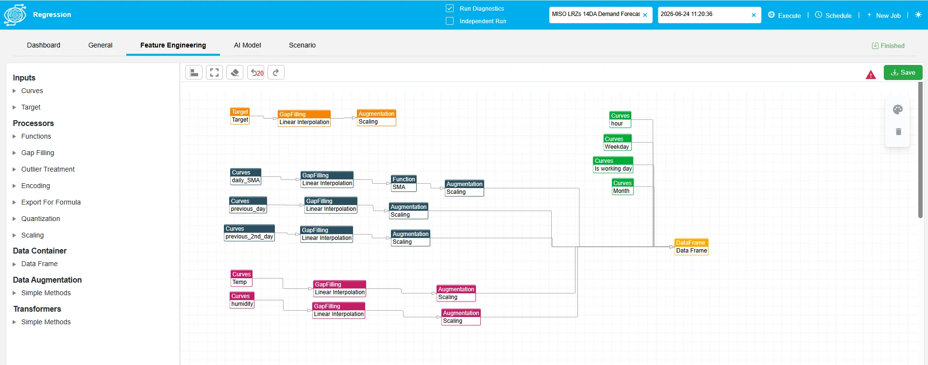
Once these coefficients have been calibrated using historical data, QR ALPS can apply the resulting profiles to forecast periods. For example, the 2025 calibrated profiles can be applied to 2026 AI demand forecasts together with the corresponding forecast temperatures to produce a 7-day-ahead (7DA) decomposition of forecast demand into base-load and weather-sensitive heating and cooling components.
5. MISO LRZ2-7 Summer Demand CDH Analysis
5.1 Data Analysis
To isolate air conditioning and cooling demand during summer months, QR ALPS as discussed in Section 2.2 of the Methodology, evaluates the cooling-sensitive component of net load:
- at : Base Load representing the temperature-independent demand component, driven by consumer schedules, diurnal human activity, day-of-week patterns, and baseline economic activity.
- CDHd,t : Cooling Degree Hour representing the cooling-sensitive component;
CDHt = max (0, Tt – CTbase )
where Tt is the temperature at the hour t.
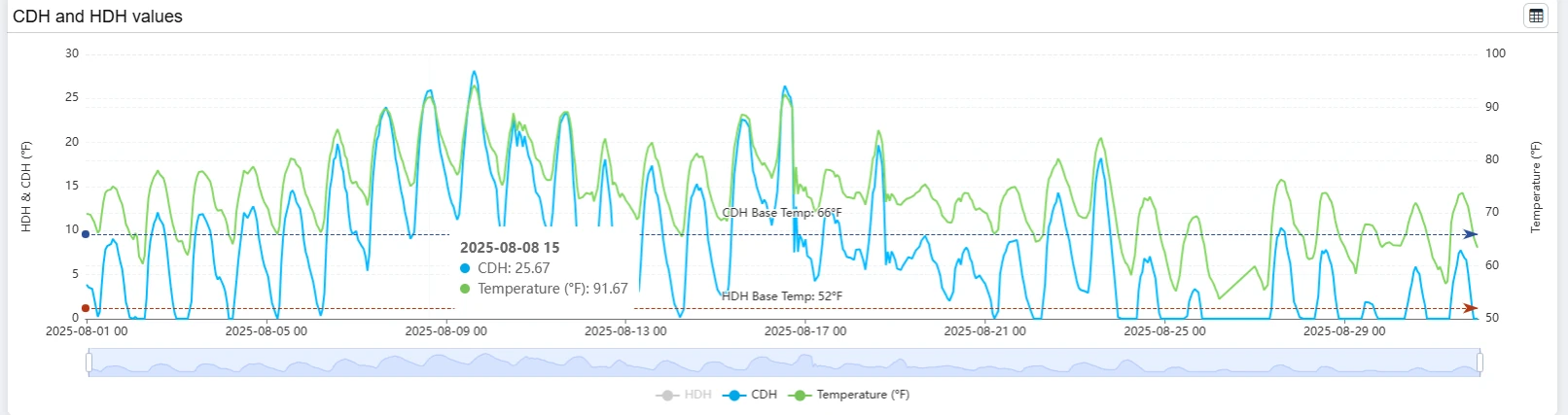
- CTbase is the cooling base temperature turning point where cooling begins, 66F.
- bt : Cooling sensitivity coefficient of the (MW/HDH). The partial derivative of net load per CDH, that is the MW change in net load per 1 unit of CDH. Unlike winter heating demand, cooling sensitivity ct peaks heavily during afternoon and early evening hours (Hours Ending 14:00 – 19:00). This reflects the compounding effect of solar radiation, heat accumulation in building masses, and peak commercial/residential HVAC utilization.
As mentioned in Section 3.1, QR ALPS is used to estimate the parameters of the load model using TRZ2-7 demand data and population weighted temperature index DTW (Detroit Metropolitan Airport) and MKE (Milwaukee Mitchell International Airport).
QR ALPS provides detailed demand decomposition analysis, separating net load into its structural base-load component and weather-sensitive heating and cooling components. The table below presents the demand decomposition at the peak-load hour of selected summer months, including the calculated Cooling Degree Hours (CDH) and the resulting heating-sensitive load component.
| Date (Summer Months) | Net Load Peak Hour | Base Load at | Cooling Sensitivity Coefficient bt | CDHt oF | CDH (MW) | Net Load (MW) |
|---|---|---|---|---|---|---|
| 2025-06-23 | 15:00 | 20,731.53 | 451.02 | 29 | 13,077.96 | 33,064.67 |
| 2025-07-28 | 13:00 | 27,103.26 | 416.10 | 20.77 | 7,951.07 | 31,691.03 |
| 2025-08-08 | 15:00 | 21,854.64 | 373.84 | 25.67 | 9,379.63 | 31,096.13 |
| 2025-09-18 | 15:00 | 21,131.97 | 343.32 | 15.30 | 5,595.55 | 24,864.77 |
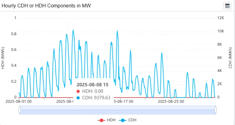
QR ALPS plots the net load and its decomposition into structural and weather-sensitive components at hourly granularity throughout the month. The MW quantities shown in the table are extracted directly from the corresponding hourly decomposition chart. The chart can be zoomed to examine any individual interval.
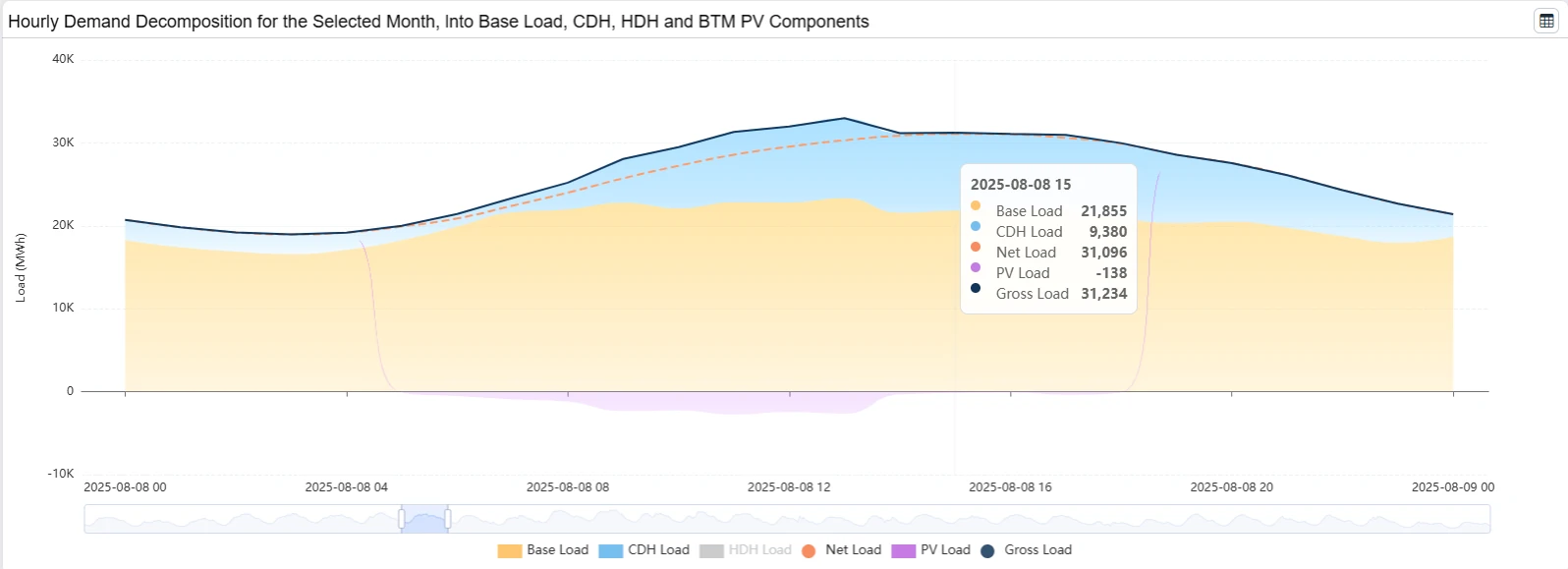
The chart tooltip displays the individual demand components and their contribution to total net load. For the 15:00 interval on August 08, the decomposition is:
| Base Load at | CDH (MW) | Net-Load (MW) |
|---|---|---|
| 21,854.64 | 9,380 | 31,096.13 |
Note that the Net-Load is the sum of the Base Load and HDH components. We next discuss these values.
5.2 QR ALPS Cooling Decomposition Methodology
5.2.1 Cooling Sensitivity Coefficient
As discussed in Section 2, the QR ALPS load model estimates and displays the parameters and quantities used in the load decomposition through multiple reports. This provides full visibility into how the heating-sensitive component is derived.
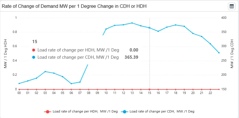
The cooling sensitivity coefficient, bt, is estimated from the historical 2025 load-temperature data. It represents the estimated marginal change in load, in MW, associated with one additional Cooling Degree Hour (CDH) at a given interval.
To stabilize the estimation, QR ALPS scales, filters, and aggregates the estimated coefficients to derive a calibrated monthly diurnal cooling-sensitivity profile, which is presented in the corresponding report. This calibrated monthly diurnal profile serves as the lookup table used to convert CDH into the cooling-sensitive MW component of demand.
For the 15:00 interval in August, the calibrated coefficient is:
b15 = 365.39.
5.2.2 Calculation of CDH
The next step is to calculate the Heating Degree Hours for the specific interval 15:00 on August 08,
- The calibrated cooling base temperature is: CTbase = 66 F.
- The temperature is: Tt = 91.67 F.
- Applying the CDH transformation, the Cooling Degree Hour for this interval are:
CDHt = max (0, Tt – CTbase ) = max (0, 91.67 – 66) = 25.67
5.2.3 Calculation of the Cooling-Sensitive MW Component
The cooling-sensitive component of net load, L(CDH,t), is then calculated using the calibrated cooling sensitivity coefficient. This is accomplished by the load model formula discussed in section 2.2:
L(CDH,t) = bt * CDHt = 373.84 * 25.67 = 9,379.63 MW
The resulting 9,379.63 MW is the model-driven cooling-sensitive component of the net load at 15:00 on August 08.
5.2.4 Application to Forecasting
The above calculation illustrates how QR ALPS performs hourly demand decomposition. The key model parameter is the calibrated monthly diurnal cooling-sensitivity coefficient, which captures how load responds to heating conditions at each hour of the day.
Once these coefficients have been calibrated using historical data, QR ALPS can apply the resulting profiles to forecast periods. For example, the 2025 calibrated profiles can be applied to 2026 AI demand forecasts together with the corresponding forecast temperatures to produce a 7-day-ahead (7DA) decomposition of forecast demand into base-load and weather-sensitive heating and cooling components.
6 AI Demand Temperature Scenario Analysis
6.1 AI Probabilistic Net-Load Forecasting
QR ALPS generates probabilistic net-load forecasts at user-defined percentiles from P1 to P99, at resolutions ranging from 5 minutes to hourly. The platform uses automated machine-learning methods to model nonlinear relationships and interactions among load drivers.
The probabilistic forecast distribution can be explored through web dashboards or exported through API. For example, P5 represents a lower-tail forecast, P50 the median forecast, and P95 an upper-tail forecast. These percentiles characterize the uncertainty distribution of the forecasted demand and answer the question:
What level of load corresponds to a given forecast percentile?
The CDH/HDH decomposition answers a different and complementary question:
What portion of the forecasted load is attributable to modeled weather-sensitive thermal demand?
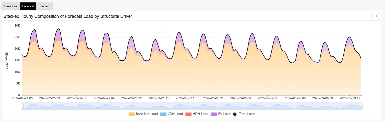
The two approaches therefore serve different purposes. Probabilistic forecasting quantifies uncertainty in the load outcome, while load decomposition explains the modeled drivers of that outcome. Combining the two enables temperature-stress scenarios to be applied consistently across the forecast distribution.
6.2 What-if-Scenario Temperature Framework
The mathematical load model was discussed in Section 2.2:
Lt = at + bt CDHt + ct HDHt − dt GHIt.
The key parameters for weather impact modeling are the marginal heating sensitivity ct (MW / HDH) and cooling sensitivity bt (MW / CDH). These were respectively estimated in Section 4 and 5 above for LRZ2-7.
In Section 2.4 we discussed how these sensitivity parameters can be used to perform temperature related what-if-scenario analysis around a baseline demand scenario. The baseline load, LBaseline, can be either historical or an AI generated forecast. The what-if-scenario framework applies identically to both cases:
Heatwave as per section 2.4:
Incremental CDH Impact:ΔCDH scenario+10,t = (CDHscenario+10,t – CDHBaseline,t ) (2.e)
Incremental MW CDH Impact:Δ L scenario+10,t = bt * ΔCDH scenario+10,t(2.c)
Total MW CDH Impact: Lscenario+10,t = LBaseline,t + Δ L scenario+10,t (2.g)
Cold-snap as per section 2.4 :
Incremental HDH Impact:ΔHDH scenario-10,t = (HDHscenario-10,t – HDHBaseline,t ) (2.f)
Incremental MW HDH Impact:Δ L scenario-10,t = ct * ΔHDH scenario-10,t(2.d)
Total MW HDH Impact: Lscenario-10,t = LBaseline,t + Δ L scenario-10,t (2.h)
When working with forecast demand, the baseline net-load forecast LBaseline is generated under the normal temperature forecast. These forecasts are however probabilistic and generate P1 to P 99 demand forecast percentiles, capturing the inherent volatility of demand, including its relationship with weather, but independently of an additional temperature shock. A scenario load forecast is applied to all 100 probabilistic forecasts.
Thus, a −10°F temperature scenario (2.h) is not itself a P95 forecast. Instead, it represents a weather shock that can be applied to P5, P50, P95, or the full P1 – P99 forecast distribution. That is the LBaseline can be the P5, P50, or P95 demand forecasts. Examples will be considered next.
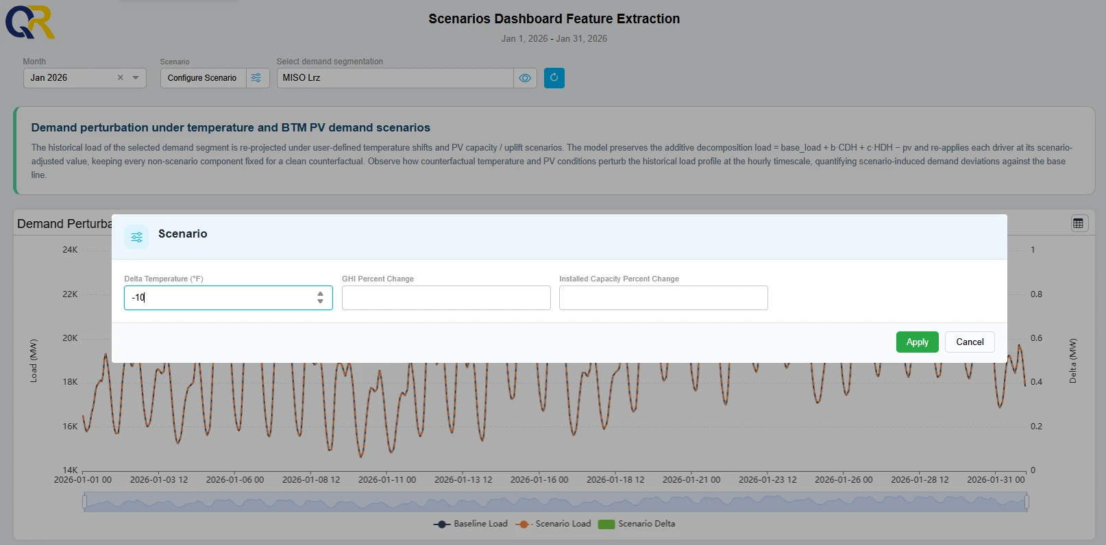
QR ALPS scenario modeling interface allows users to define weather and PV scenario shocks by specifying the corresponding change.
6.3 From Temperature Change to a Diurnal Profile
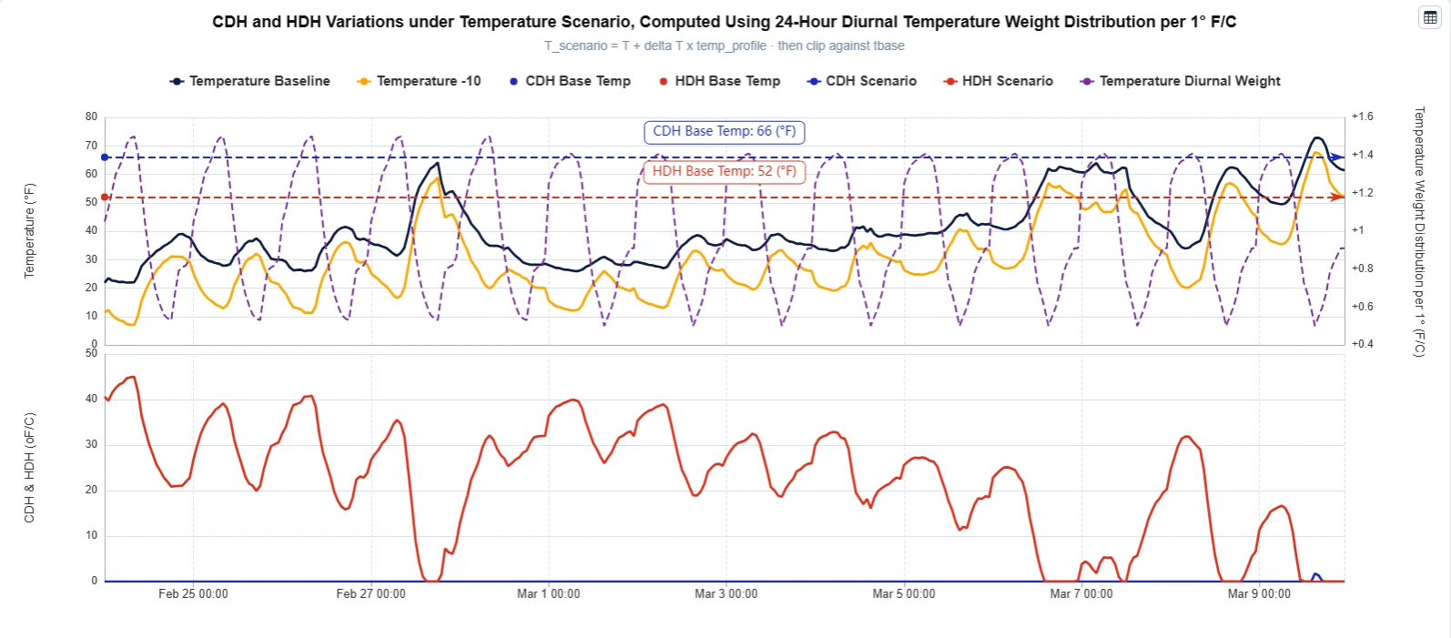
To apply a temperature shock ΔT (e.g., ± 10o For C) to a temperature, be it an actual or a forecast, the actual temperature degree changes are not uniformly distributed across the hours. Early morning and late night cold impacts are more pronounced than midday impacts. Rather than applying a uniform temperature change, QR APLS employ a dimensionless diurnal profile Temp_Profile describing how the nominal shock is distributed across 24 hours, while respecting the diurnal colder and warmer pattern.
This is then used to apply the temperature shift ΔT to the (actual or forecast) temperature TBaseline to derive the temperature under the scenario, TScenarioΔT:
TScenarioΔT = TBaseline + ΔT * Temp_Profile (6.a)
Then the TScenarioΔT is used in computing HDHScenarioΔT and CDHScenarioΔT:
CDHScenarioΔT,t = max (0, TScenario ΔT,t – CTbase ) (6.b)
HDHScenarioΔT,t = max (0, HTbase – TScenarioΔT,t )(6.c)
These are then used in (2.e) and (2.f) to define the corresponding Incremental CDH and HDH changes.
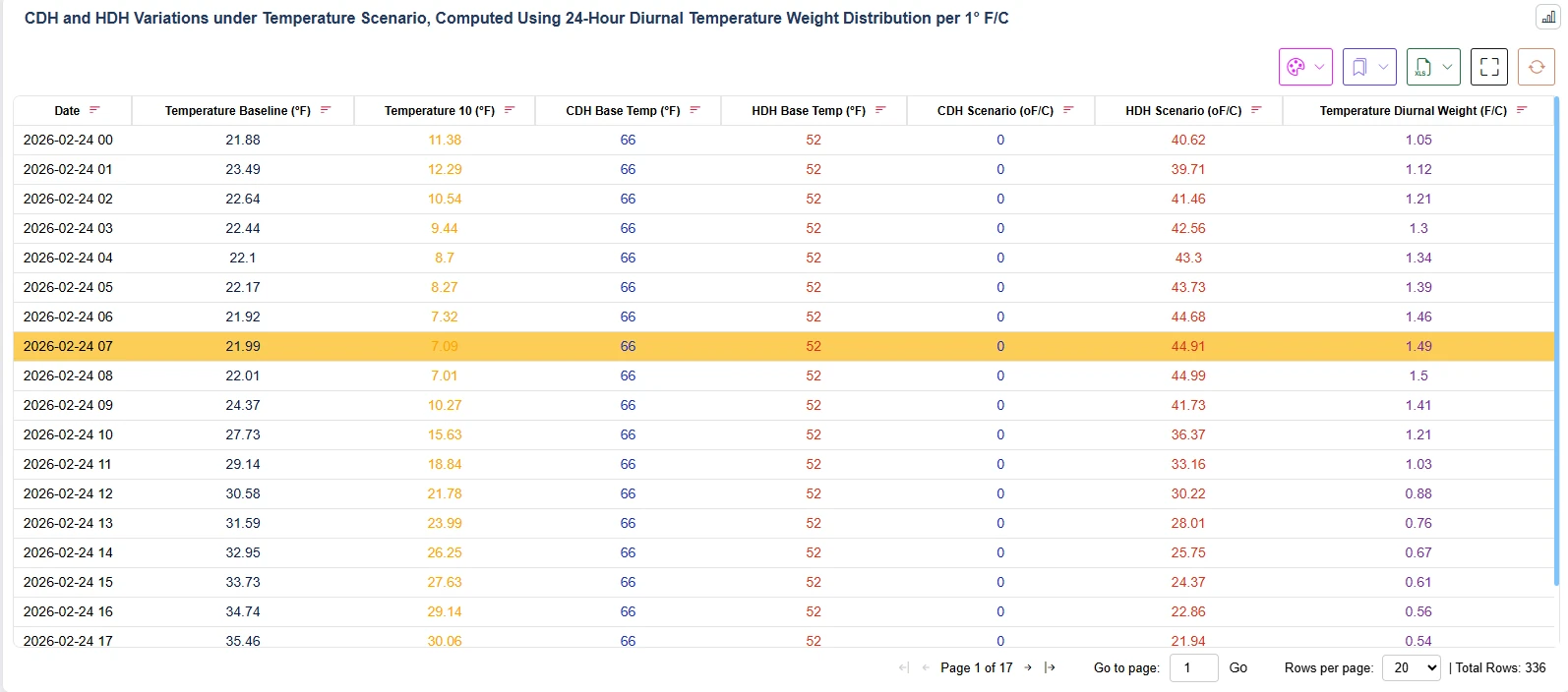
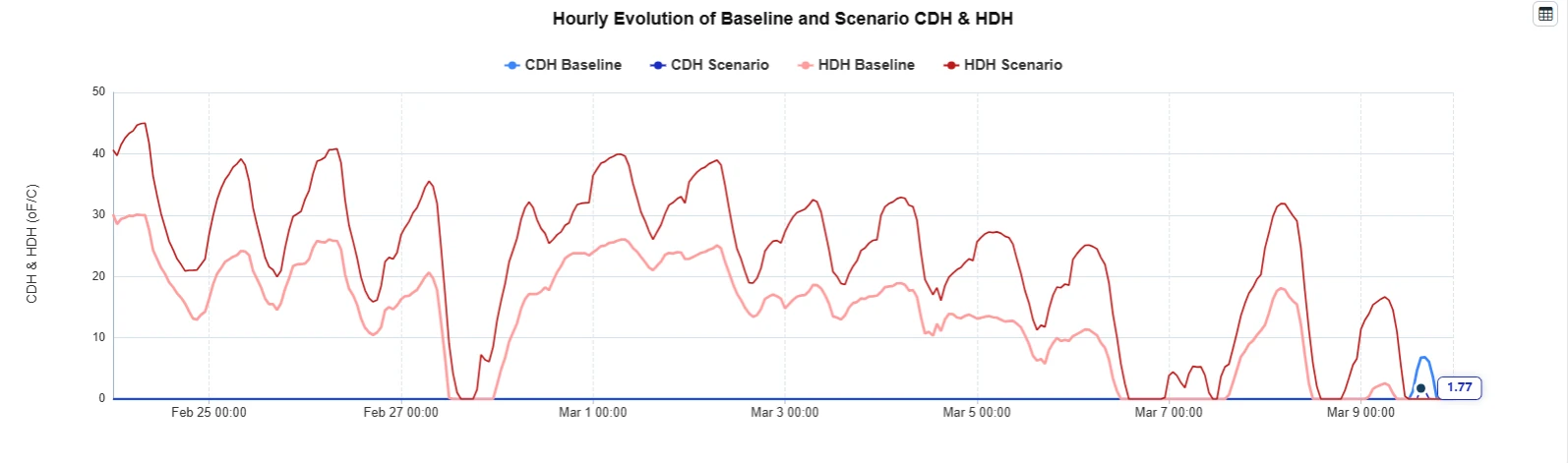
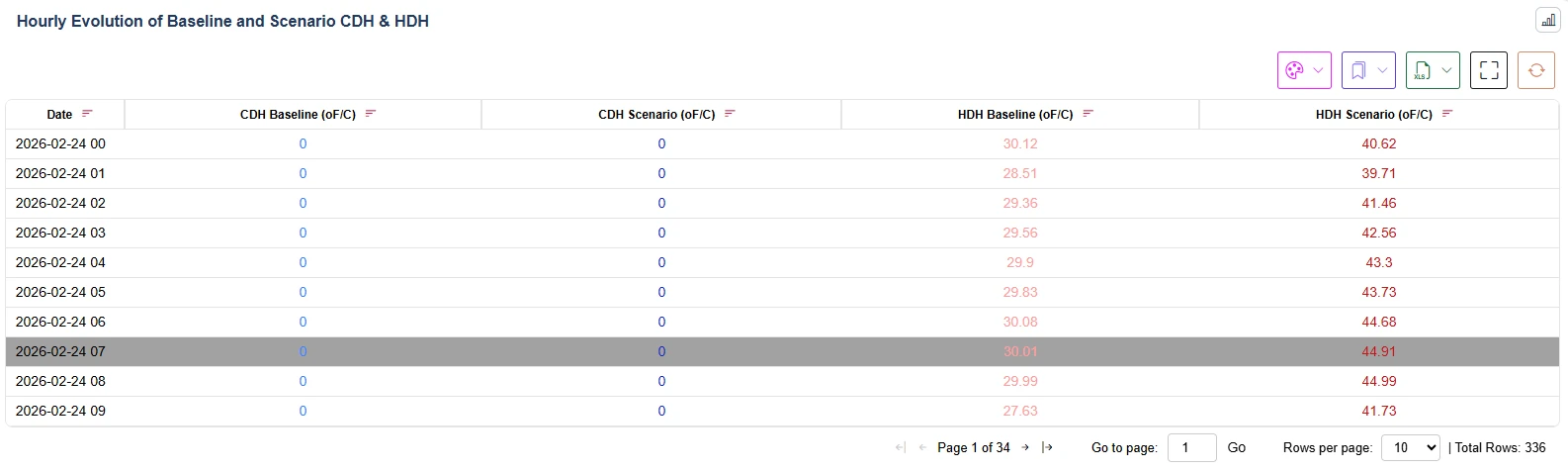
The resulting baseline and scenario temperatures, HDH and CDH values are made available through QR ALPS reports, providing full visibility into how the temperature scenario propagates into the load forecast:
6.4 Cold Snap Scenario Analysis
Extreme winter weather events can produce substantial and nonlinear increases in electricity demand. A cold-snap scenario allows traders, planners, utilities, and risk managers to quantify the incremental demand and associated hourly load impacts under a specified temperature shock.
6.4.1 Modeling Temperature Shock Profile
Consider a −10°F temperature scenario. QR ALPS first distributes the temperature shock across the 24-hour period using the method Temp_Profilet. The scenario temperature and corresponding HDH and CDH values are then calculated using the equations in section 6.2, and 6.3.
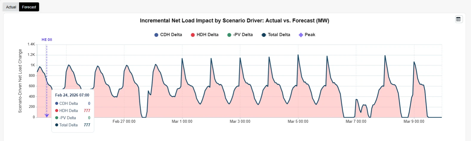
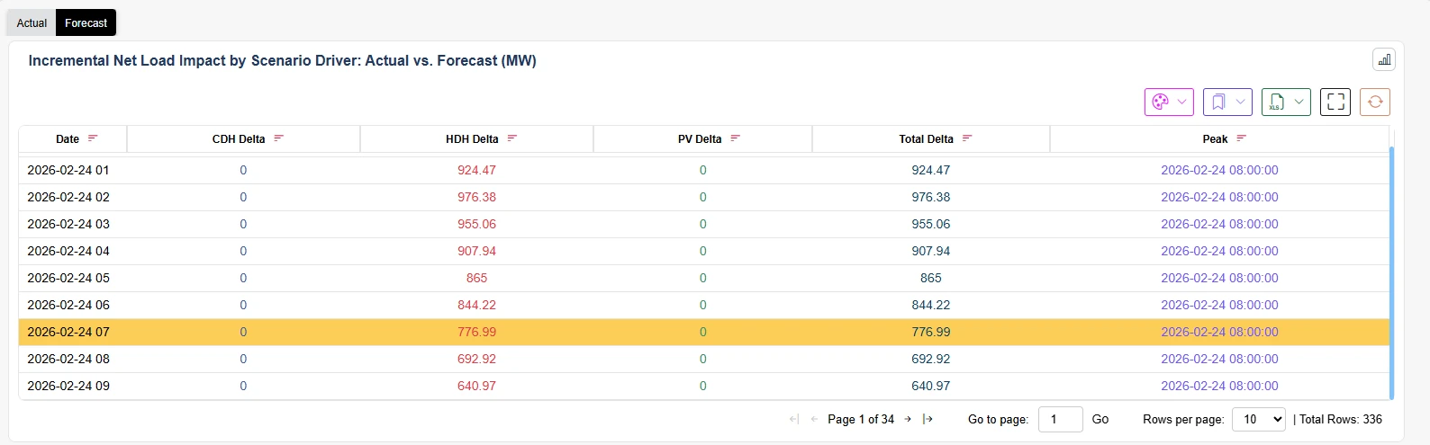
For the MISO LRZ2-7 example, a day-ahead forecast is generated at 07:00 on February 23, 2026, for February 24, 2026. The analysis applies a ΔT = −10°F temperature stress scenario to the forecast.
For the February 24, 07:00 interval:
| Temp_Profile07 | Estimated HTbase | (Forecast) TBaseline,07 | ΔT |
|---|---|---|---|
| 1.49 F | 52 F | 21.99 F | -10o F |
where the scenario inputs Temp_Profile07 (1.49F) and HTbase (52F) are estimated by the load model.
Therefore, the forecast weather scenario under the -10 F shock becomes
TScenario-10F,07 = TBaseline – (10 * Temp_Profilet) =
TBaseline,07 + (-10) * 1.49 = 21.99 – 14.9 = 7.09 F
Substituting the stressed weather, we derive HDHScenario-10F,07:
HDHScenario-10F,07 = max (0, HTbase – TScenario-10F,t ) =
max (0, HTbase – TScenario-10F,07 ) = max (0, 52 – 7.09) = 44.91
Furthermore, baseline HDH is computed as
HDHBaseline,07 = max (0, HTbase – TBaseline,07) =
max (0, 52 – 21.99) = 30.01
Therefore,
ΔHDHScenario-10F,07 = 44.93 – 30.01 = 14.90
6.4.2 The Demand Under Temperature Shock Profile
For 7:00 am, QR ALPS model estimates the heating sensitivity coefficient to be
c(07:00) = 52.09 MW/HDH.
Finally, the net load scenario corresponding to the -10F shock to the baseline load forecast (such as the median P50 or high P95 profile) is given by:
The incremental demand attributable to the temperature shock is by (2.d):
Δ L scenario-10,07 = ct * ΔHDH scenario-10,07 = 52.09 * ( 14.92 ) = 776.14 MW
The total MW demand attributable to the temperature shock is by (2.h):
Lscenario-10,t = LBaseline,t + Δ L scenario-10,t = 20,396 + 776.14 = 21,172.14 MW
The same calculation can be applied independently to P5, P50, P95, or any other percentile of the probabilistic forecast distribution.
Because both the heating sensitivity coefficient and the temperature-shock profile are calibrated as diurnal patterns, the model can represent different load responses across the hours of the day. This provides traders, utilities, and system operators with hour-by-hour visibility into the incremental demand, ramping requirements, and potential system stress associated with an extreme temperature scenario.
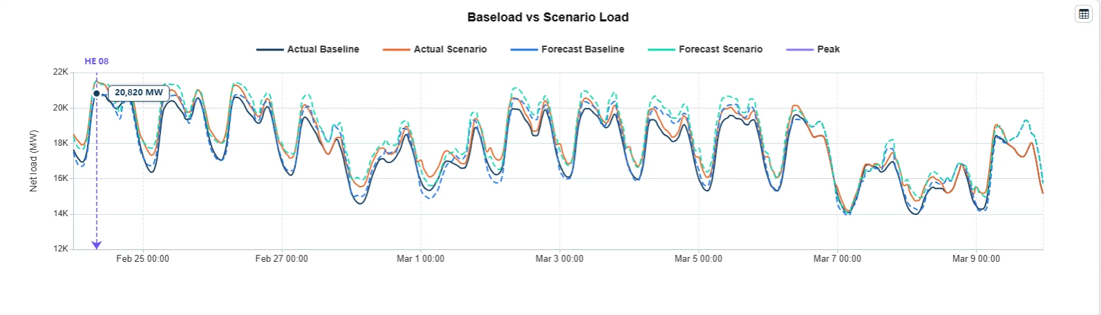
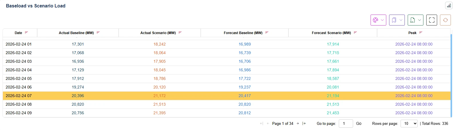
QR ALPS provides the baseline and scenario temperatures, HDH/CDH values, sensitivity coefficients, component MW values, and resulting net-load forecasts through multiple analytical reports.
The analysis can also show the relative contribution of the modeled load components under the temperature scenario. For this case study, the analysis isolates the effect of the temperature change while keeping all other forecast inputs unchanged; specifically, the PV scenario and other non-temperature-related components remain constant between the baseline and temperature-stress cases.
6.5 Summer Heatwave Scenario Analysis
Extreme summer weather can produce substantial increases in electricity demand, particularly as cooling requirements rise. A heat-wave scenario allows traders, planners, utilities, and risk managers to quantify the incremental demand and associated hourly load impacts under a specified temperature shock.
6.5.1 Modeling Temperature Shock Profile
Consider a +10°F temperature scenario. QR ALPS first distributes the temperature shock across the 24-hour period using the method Temp_Profilet. The scenario temperature and corresponding HDH and CDH values are then calculated using the equations in section 6.2, and 6.3
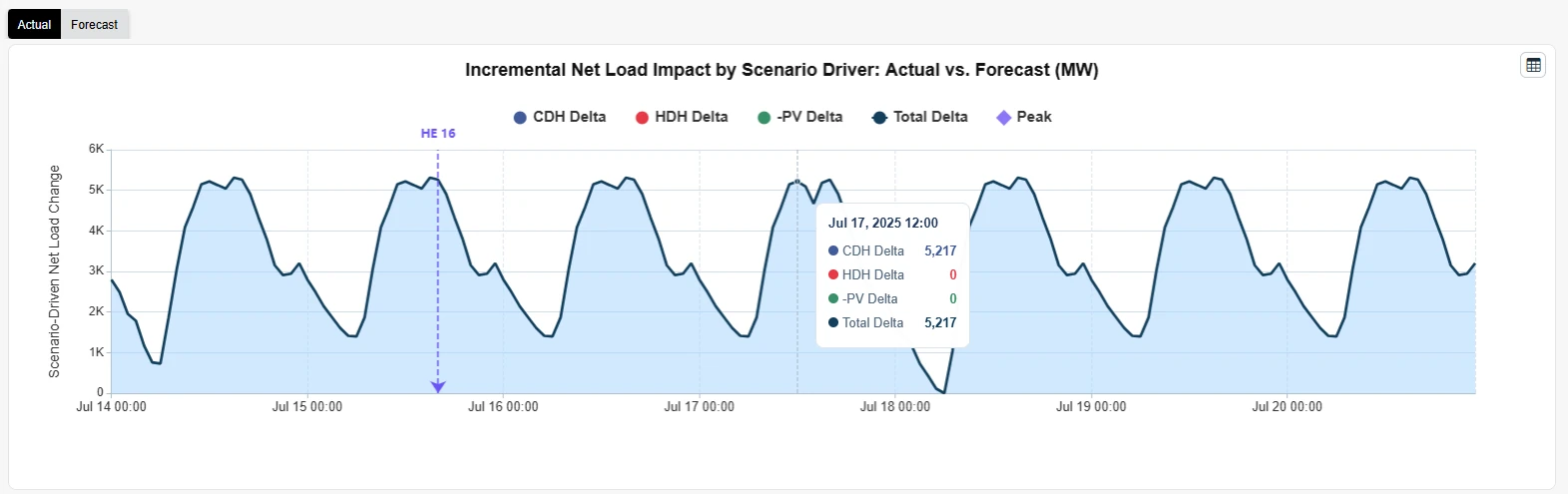
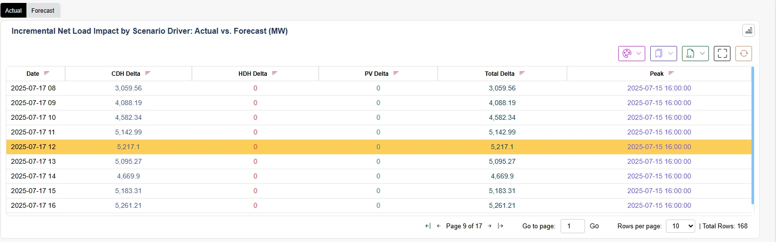
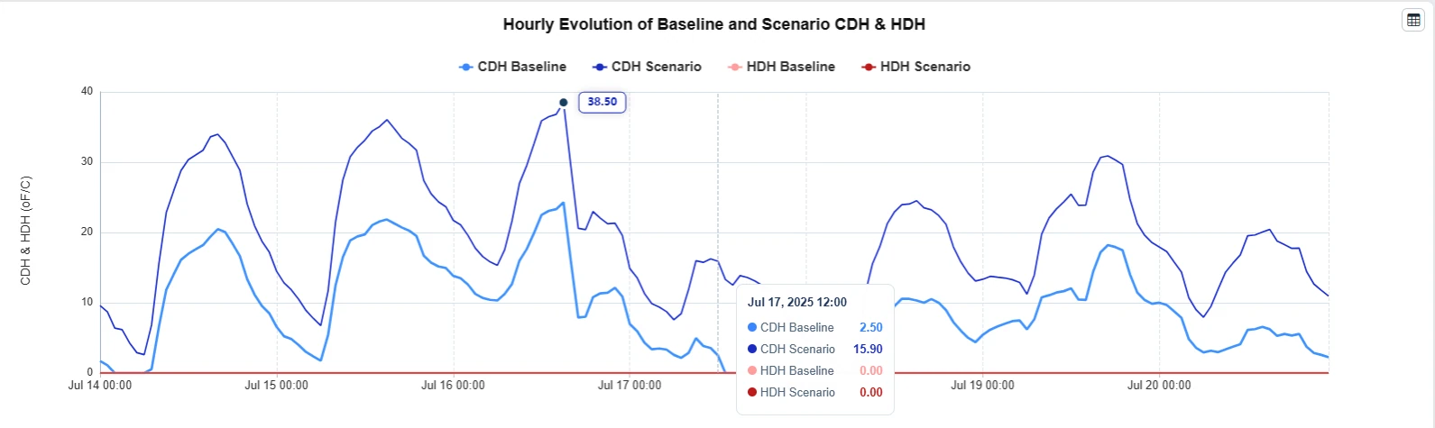
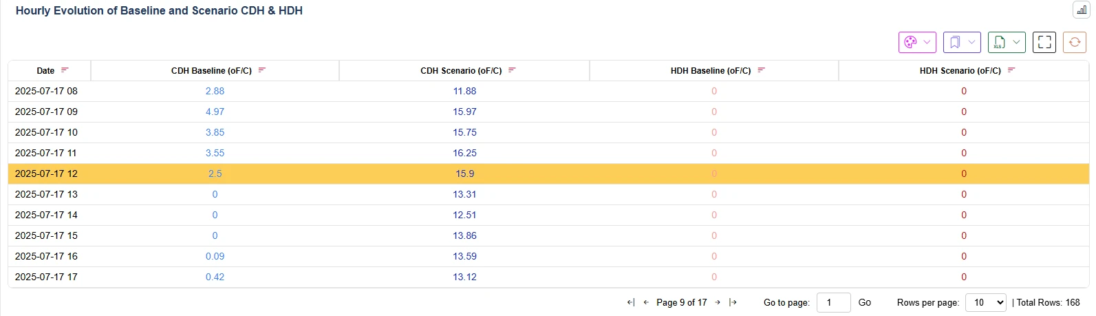
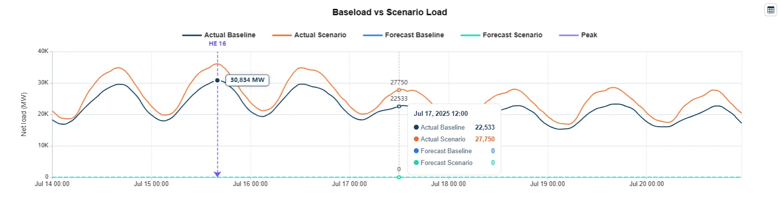
For the MISO LRZ2-7 example, consider the exact date and time of 12:00 noon on July 17, 2025. The analysis applies a ΔT = +10°F temperature stress scenario to this point.
For the July 17, 12:00 noon interval:
| Temp_Profile12 | Estimated CTbase | (Forecast) TBaseline,12 | ΔT |
|---|---|---|---|
| 1.34 F | 66 F | 68.50 F | +10o F |
where the scenario inputs Temp_Profile12 (1.34F) and CTbase (66F) are estimated by the load model.
Therefore, the forecast weather scenario under the +10 F shock becomes
TScenario+10F,12 = TBaseline,t + (10 * Temp_Profilet)
= TBaseline,12 + (10) * 1.34 = 68.50 + 13.4 = 81.9 F
Substituting the stressed weather, we derive CDHScenario+10F,12:
CDHScenario+10F,12 = max (0, TScenario+10F,t – CTbase ) =
max (0, TScenario+10F,12 – CTbase ) = max (0, 81.9 – 66) = 15.9
Furthermore, baseline CDH is computed as
CDHBaseline,12 = max (0, TBaseline,12 – CTbase ) =
max (0, 68.50 – 66) = 2.5
Therefore,
ΔCDHScenario+10F,12 = 15.9 – 2.5 = 13.4
6.5.2 The Demand Under Temperature Shock Profile
For 12:00 noon, QR ALPS model estimates the cooling sensitivity coefficient to be
b(12:00) = 389.34 MW/HDH.
Finally, the net load scenario corresponding to the +10F shock to the baseline load forecast (such as the median P50 or high P95 profile) is given by:
The incremental demand attributable to the temperature shock is by (2.c):
Δ L scenario+10,12 = bt * ΔCDH scenario+10,12 = 389.34 * ( 13.4 ) = 5,217.156 MW
The total MW demand attributable to the temperature shock is by (2.g):
Lscenario+10,12 = LBaseline,12 + Δ L scenario-10,12 = 22,533 + 5,217.156 = 27,750.156 MW
The same calculation can be applied independently to P5, P50, P95, or any other percentile of the probabilistic forecast distribution.
Because both the cooling sensitivity coefficient and the temperature-shock profile are calibrated as diurnal patterns, the model can represent different load responses across the hours of the day. This provides traders, utilities, and system operators with hour-by-hour visibility into the incremental demand, ramping requirements, and potential system stress associated with an extreme temperature scenario.
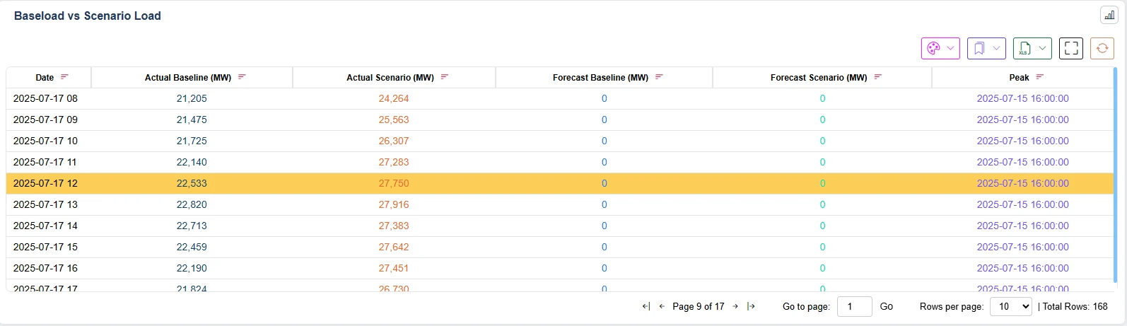
QR ALPS provides the baseline and scenario temperatures, HDH/CDH values, sensitivity coefficients, component MW values, and resulting net-load forecasts through multiple analytical reports.
The analysis can also show the relative contribution of the modeled load components under the temperature scenario. For this case study, the analysis isolates the effect of the temperature change while keeping all other forecast inputs unchanged; specifically, the PV scenario and other non-temperature-related components remain constant between the baseline and temperature-stress cases.